
 , Peijian Shi2, Diego Caratelli3
Revised 29 July 2022
Accepted 1 August 2022
Available Online 17 August 2022
- DOI
- https://doi.org/10.55060/j.gandf.220817.001
- Keywords
- Gielis Transformations
Power laws
Conic section
Natural shapes - Abstract
A uniform description of natural shapes and phenomena is an important goal in science. Such description should check some basic principles, related to 1) the complexity of the model, 2) how well its fits real objects, phenomena and data, and 3) a direct connection with optimization principles and the calculus of variations. In this article, we present nine principles, three for each group, and we compare some models with a claim to universality. It is also shown that Gielis Transformations and power laws have a common origin in conic sections.
- Copyright
- © 2022 The Authors. Published by Athena International Publishing B.V.
- Open Access
- This is an open access article distributed under the CC BY-NC 4.0 license (https://creativecommons.org/licenses/by-nc/4.0/).
1. INTRODUCTION
Mathematics is a crowning achievement of humanity and a triumph of the human mind. It is also the language of science with a continous interplay between algebra, analysis and geometry. In the early 17th century, the Scientific Revolution was initiated by a uniform description of natural phenomena in terms of the classic conic sections, which had been studied in antiquity. Galileo Galilei (1564–1642) found that the parabola describes the trajectory of free moving objects in the earth’s gravitational field, and Johannes Kepler (1571–1630) showed that the orbits of planets are ellipses. Building on these foundations, Isaac Newton (1643–1727) developed methods based on isotropic spaces with the Euclidean circle, to deal with the anisotropy of the other conic sections, which are projective equivalent to the circle. Newton brought the ideas of the Ancient Greek mathematicians back to center stage. Indeed, our main methods in science are straight lines and circles, and we measure deviations from these two main tendencies (curvature in its manifold disguises). One major consequence was the development of mathematical physics with solutions to general problems in physics in terms of (partial) differential equations.
The Scientific Revolution led to great successes in physics, but also to a difficult relationship with biological objects and phenomena. Historically, common strategies have been to apply results from physics to biology by inference (and chemistry). However, the abstraction that proved successful for physics is no guarantee for success. Not so long ago Marcel Berger wrote explicitly [1]: “Present models of geometry, even if quite numerous, are not able to answer various essential questions. For example: among all possible configurations of a living organism, describe its trajectory (life) in time”.
A different strategy is to search for a uniform description of biological shapes and phenomena, which encompasses the conic sections, as generalization of the circle. It is widely believed that such a universal description for the wide variety of biological shapes in our everyday world (and more generally natural forms) does not exist, but recent botanical and biological research suggests otherwise.
Botany and biology may then be the next step, but a uniform description is only the first step. Any method with a claim to universality must be transformed into a full-fledged scientific methodology, linked to existing mathematics and going beyond plants and botany. This raises the intriguing question of what is or should be a universal formula? What criteria must a universal equation meet? An important principle is the Universality Principle: Universality reminds us of Newton and our successful 20th-century theories for the large and the small, so, how far can a formula or equation be applied?
Using the past as our guide, this description will need to be closely related to conic sections and the circle, it will have to fit many observables in nature, and it will need to be connected to fundamental geometry and mathematical physics. To this end, nine guiding principles are proposed, in groups of three. The first group is related to the simplicity of the model; the second to how well it fits real data and the third deals with the relation to mathematical physics.
We discuss three examples.
First, allometry in natural phenomena, animals and plants. Starting as a theory of relative growth [2], a wide range of publications in the past 25 years have focused on allometry in plants, animals, ecosystem and even urban cities. The work of West, Brown, and Enquist (and the WBE equations) in the 1990s led to numerous articles on allometry in biology [3–6]. In the past twenty years an enormous amount of empirical allometry relationships have been unveiled in biology at all levels, from the giant to the small, and for living and non-living. It has been called a theory of everything.
Second, superellipses and their generalisation as Gielis Transformations, a generic geometric transformation that unifies a wide variety of abstract and natural shapes, including polygons, tree rings, flowers, plant leaves and seeds, seastars, and diatoms [7–14]. Gielis curves, surfaces, and transformations GT provide for a uniform description of natural shapes at all levels and scales. It was called “Universal Natural Shapes” [15,16], and “A magic formula of Nature” [17] and when the original article [7] was published, the website of the American Mathematical Society wrote: “A botanical Kepler awaiting his Newton”.
A third example is a recent universal formula for describing the shape of bird eggs, hereafter referred to as the NRG equation [18]. The NRG equation is not only presented as a mathematical formula to fit all types of avian eggs into one formula but it is also promoted as a universal equation for bird eggs. By far, most eggs tend to be spherical, ellipsoidal, or ovoid, but the pear-shaped form is observed in the eggs of Common Guillemots (Uria aalge). Stoddard et al. [19] have shown that two biologically relevant parameters, asymmetry, and ellipticity, are sufficient to quantify egg shape diversity. The concept of asymmetry is a relative measure that indicates the deviation from a circle or ellipse in one direction since all eggs exhibit bilateral symmetry in their cross-section from top to bottom. Avian eggs are an example of going from spherical isotropic geometry to anisotropy in one direction.
Before listing the nine principles it should be noted that usefulness or applicability is perhaps the least interesting criterion from a mathematical point of view, at least as a starting point. Typically, there are various ways to develop formulas to describe shapes and phenomena. Various equations for bird eggs have been reviewed recently [20], and there are many more [21,22]. The main goal should be to apply mathematics to the natural sciences in the best possible way. Best is always a relative term, but in our view, in deriving a general equation for many (or any) natural shapes or phenomenons, there are at least nine principles, divided into three groups.
2. A LIST OF PRINCIPLES FOR UNIVERSAL EQUATIONS
2.1. The First Group of Three Principles
This relates to compact and simple descriptions.
P1. Oresme-Newton Principle. This refers to the least deviation from a circle or the Pythagorean theorem. In his work, Isaac Newton (1643–1727) incorporated Kepler’s laws and the work of Galileo into a coherent framework. The circle as a measure of deviations from straight lines, proposed by Nicolas Oresme (c1320–1382), became fundamental in all fields of science. Following Newton’s principle, the most mathematically elegant way to develop methods for studying anisotropic shapes is to start from a circle and the notion of isotropy (equal in all directions), in the spirit of Pythagoras. Eggs are slightly anisotropic in one direction but retain their bilateral symmetry in one plane and their circular symmetry in the perpendicular plane.
P2. Hein Principle on single curves, named after the Danish mathematician Piet Hein (1905–1996). In the 1960s, architects redesigning Sergel’s Torg in Stockholm were looking for an aesthetically pleasing shape to optimize both the available space for an underground shopping center and traffic flow. They devised a shape in between an ellipse and a rectangle, composed of various arcs and lines, but mathematician Piet Hein informed the architects that their solution could be considered as a single curve, a superellipse [23] defined by:
These curves were first considered in full generality by Gabriel Lamé (1795–1860) to model the shape of crystals [24]. A single mathematical equation and pure mathematical elegance; a generalization of Pythagoras and the circle defining a family of curves including circles and conic sections, ellipses, diamonds and squares, rectangles and diamonds, and all shapes in between. It is derived from the equation of a circle, but this is only historically so; in fact, the Euclidean circle should be considered as a special case. In three dimensions, spheres and cubes, ellipsoids and beams, cylinders and supereggs result [25,26]. For any value of n, special trigonometric functions can be derived, and a generalized Pythagorean Theorem of the form
Gielis curves further generalize Lamé-curves avoiding the limitation of symmetry of superellipses. When transforming supercircles into polar coordinates, the introduction of symmetry parameter m allows the orthogonal axes to fold in and out like a fan, determining the number of fixed points on a circle [7].
P3. Arnold-Oleinik Principle is named after the Russian mathematicians Vladimir I. Arnold (1937–2010) and Olga A. Oleinik (1925–2001). The simpler the model and its derivatives are, the better, in the spirit of Ockham’s principle. According to V.I. Arnold [27], “Complex models are rarely useful”. In mathematical terminology [28]: “What is essential for the topological complexity of an object is not the degree of the equation, but rather the number of monomials that appear in the polynomial with nonzero coefficients. Thus, we have the problems of oligomials, i.e., the topology of objects specified by polynomials of arbitrarily large degree but with a restricted number of monomials.” Eq. (1) is, of course, an excellent example of a trinomial in two variables, with one control variable, the exponent n. This principle prefers compact descriptions over expansions or polynomials.
2.2. The Second Group of Three Principles
This determines how reliable a model equation fits real data and objects, whether it is the best possible fit for individual objects and groups of objects, and how widely applicable the model with claims to universality is.
P4. Gauss-Chebyshev Principle is named after Carl Friedrich Gauss (1777–1855) for his method of least squares and Pafnuty Chebyshev (1821–1894), who searched for the best possible coordinate system fit to shapes (historically the origin of Chebyshev polynomials). Do universal equations also provide the best possible fit? Does this result in the best possible coordinate system adapted to shape? In recent years, for example, superellipses have proven to be excellent methods for describing a variety of natural shapes, as we will show below.
P5 A and B. Two Feynman Principles on complete sharing of experimental data and critical thinking, named after Richard Feynman (1918–1988). Since it is easy to be fooled by overconfidence in one’s models, Principle 5A states that rigorous testing and experimentation are key, especially by other researchers. Principle 5B states that all data, including the methods used, must be made available to other scientists to test the limitations of the methods. It is important for progress in science that others can test and verify hypotheses and results.
P6. Universality-Unity Principle: If an equation works in one domain, does it work in other domains? For other shapes? For the small and the large? How “universal” is it? What is relevant to the natural sciences is not only how it can describe a quantity at the statistical level, but also individual forms, including outliers (Whether it holds in 97 dimensions is a mathematical question and less relevant here). Obviously, the higher it universality score (bringing more and more natural shapes and phenomena under the same umbrella), the higher it scores on the scale of unification. Full unification with the focus on shapes is the geometrical version of Pythagoras’ “All is number”.
2.3. The Third Group of Three Principles
This determines how closely the model is related to mathematical physics and the computational complexity.
P7. Fourier-Lamé Principle of mathematical physics. Does it generate analytical solutions to classical boundary value problems? The names Joseph Fourier (1768–1830) and Lamé refer to the Fourier series solution of the heat equation and elasticity theory, respectively. The Laplacian is a key element in most common boundary value problems BVP, such as the Laplace, Helmholtz, Poisson, and Schrödinger equations. A 20th-century name that can be added here is Alan Turing (1912–1954), because of his chemical basis of morphogenesis [29]. In the spirit of Gabriel Lamé’s Unique Rational Science, P4 is closely linked to P7: having best-fit coordinate systems adapted to the shape, one can then solve the relevant BVP on this system.
P8. Laplace-Plateau Principle of Shape Optimization. Another way of thinking about growth concerns the optimal shapes for certain natural curvature conditions. It bears the name of Pierre-Simon Laplace (1749–1827) for capillary forces and the Laplacian, and Joseph Plateau (1801–1883), who studied soap films. A key inequality is K ≤ H2, with K the Gaussian curvature and H the mean curvature. Well-known are Delaunay’s surfaces of revolution with constant mean curvature CMC (catenoids and planes for H = 0; spheres, nodoids and unduloids for H ≠ 0. A remarkable geometrical fact is that the curves defining the rotational CMC surfaces are the conic sections). This principle involves various maximum or minimum principles.
P9. Principle of Computability. A simple formula that would take ages to compute is not what we strive for. Ideally, the computational methods should align with methods already available. Eq. (1) presents its own mathematical challenges (the Last Theorem of Fermat and Lamé curves are very closely related) but it opened the door to the application of Fourier projection methods to solve a variety of boundary value problems on very different domains [30]. There are also direct connections with special polynomials, as will be shown further.
The focus on geometry is intentional because “While algebra and analysis form the foundations of mathematics, geometry is the core” [31]. Shiing-Shen Chern (1911–2004) saw two major tasks for the geometry of the 21st century: first, the extension of geometry with polyeders, polyhedrons, and piecewise-linear structures, to combine the differences and differentials into one framework. Second, is the extension of Riemannian geometry with Finsler geometry, which he called “Riemannian geometry without the quadratic restriction” [32]. Eq. (1) can play an important role, as the simplest examples of Lamé-Minkowski and Riemann-Finsler geometries, and because squares and diamonds are special cases of Eq. (1).
3. ALLOMETRY, NRG AND THE PRINCIPLES
Allometry clearly checks all the boxes in Groups 1 and 2, namely a simple model with a lot of data to support the claims to universality, since it applies to the small and the great, and much in between. More details will be discussed further in Section 6.
Let us now see how the NRG and other egg variants fit in with these principles. Starting from the Pythagorean Theorem
When f (x) = T = 1 it is a circle, and f (x) = T < 1 yield an ellipse with its long axis horizontal. The next simplest function gives Preston’s Simple Ovoid:
For pyriform egg shapes a cubic equation is used, Preston’s Alcid Ovoid:
For all practical purposes, T, a, b and c give an excellent fit, and these four parameters perfectly capture the shape of an egg better than other equations [20].
Preston’s formulas and Lamé’s superellipses (Eq. (1)) satisfy P1, P2, and P3. Simple and easy curves, as a generalization of the Pythagorean theorem, and curves defined by a single equation and low topological complexity. On the other hand, NRG is a composition of single curves [18], but it cannot be considered simple in any sense of the word, violating P2 and P3.
In the NRG equation the four parameters L, B, w and DL/4 relate to real measurements of direct use on avian eggs and poultry. The same is true for the parameters T, a, b, c in the Preston equation. Concerning P6, both the Preston formula and the NRG equation are limited by their definitions and cannot handle many other natural forms, and cannot fit superellipses. They may find use in a few unrelated fields, such as pear-shaped atomic nuclei [33]. Moreover, [18] presents the formula without fitting it to real eggs. As a pure description it does not check the second group or third group of principles.
4. GIELIS TRANSFORMATIONS AND THE PRINCIPLES
The limitation of Eq. (1) is that it can only represent a limited number of shapes with the symmetry of diamonds, squares, and rectangles. The generalization to Gielis Transformations GT (Eq. (3)) widens the descriptive potential of superellipses. They can act as a transformation on planar functions f (θ). When this is a constant function R, GT transform the circle with radius R.
In Eq. (3) Gielis Transformations are a generalization of superellipses describing a much wider range of abstract and natural shapes. By transforming supercircles into polar coordinates, they can deal with any symmetry by introducing the symmetry parameter m.
The parameter
4.1. P1-P3: Complexity of the Model
As a generalization of the Pythagorean Theorem, Gielis transformations correspond to Principles P1, P2, and P3. To model natural shapes the number of parameters can generally be reduced to four or even to one or two (in the special cases of circles and ellipses). Even when the full six parameters are used, all supershapes form a six-dimensional manifold only.
The original expression is in polar coordinates but can be rewritten into algebraic form because of the natural connection between cos(mθ), sin(mθ) and Chebyshev polynomials of the first and second kind, respectively. Hence shapes can be expressed both in polar form and as algebraic polynomials [12]. Fig. 1 shows the closure of this scheme.
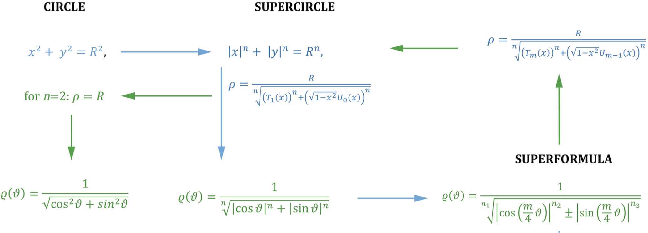
Closure of the scheme.
4.2. P4-P6: Modeling, Experimental Data, and Universality
Regarding the second group of principles, GT has been tested on over 40000 biological samples over the last decade [9–13,34] and proved to be an excellent model (P4-P5). Tested rigorously with the appropriate statistical methods, it was shown that GT fit many natural shapes very well. In the seminal article on tree rings [9] a simplified version with fewer (two) parameters of Eq. (3) was compared with methods based on circles. The two methods were compared with Aikake Information Criterion AIC and Bayesian Information Criterion BIC. These criteria allow for comparing methods based on their efficiency (how well it performs) and the number of parameters. Both AIC and BIC confirmed the superiority of GT over methods based on circles [9]. In softwoods, the tree rings closely resemble circles (see Fig. 2), but this is misleading: they are superellipses. In Fig. 2 one can observe supercircular shapes in white cedar.
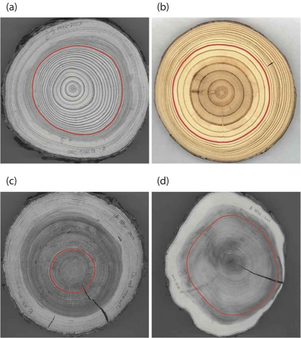
Superelliptical tree rings in softwoods. (a) Jack pine (Pinus banksiana), (b) red pine (Pinus resinosa), (c) tamarack (Larix laricinia) and (d) white cedar (Thuja occidentalis) [9].
Importantly GT opens doors to unification and geometrization of natural form linking the description of shape to optimization principles. At the same time, a full methodological method has been developed for science, validating GT as a valuable experimental tool. More and more natural shapes can be described with GT, including avian eggs as proposed in [35].
In the experimental sciences, it is data that matter, for the Gielis equation as well as for the NRG equation.
In Eq. (3) there are six parameters need to be fitted: m, A, B, n1, n2, n3. For closed non-intersecting curves, the parameter m is an integer, which determines the number number of fixed, equally spaced points on a circle. To reduce the complexity of the model in depicting avian egg shapes, we propose a new simplified version where m is fixed to be 1,
The choice for m = 1 is because, in bird eggs, one observes mirror symmetry in one direction and asymmetry in the perpendicular (longest) direction. It has already been established that the simplest geometric way to produce such mirror symmetry in one direction and asymmetry (up and down) in the other direction is a monogon with m = 1 [35]. By choosing appropriate values for the exponents in the one-angles or monogons, a whole range of eggs can be described. The description of egg shapes in 3D as a surface of revolution or with slight deviations from circular symmetry is straightforward.
In [36] conclusive evidence is presented that SGE-1 (Eq. (4)) is a much better model than the NRG, even with one parameter less. Moreover, the goodness-of-fit of the NRG, which is not a best-fit (P4), depends on the estimation of the principal axis by SGE-1, since the complexity of Eq. (2), prohibits directly estimating the parameters of the NRG [36]. Although the NRG equation models the eggs reasonably well, it is not Chebyshev-proof.
P5: The full methodology, data, and results have been made available in the various published articles and as supplementary information [9,10,34,37–39]. The complete R-software has been published in full on the Comprehensive R Archive Network CRAN [40]. Other researchers have used GT independently in modeling petioles and understanding the relation of form to resistance against bending and twisting [41].
P6: Universality of GT in nature will be discussed in the final section, but it is remarked that the original article [3] has been cited over 570 times to date in a variety of fields in mathematics, physics, psychology, biology, education, and various fields of technology and engineering. The first and third author co-founded The Antenna Company, where Eq. (3) is key to new antenna designs and fast computational methods [42–53].
4.3. P7-P9: Mathematical Physics and Computations
Regarding P7, once a best-fit coordinate system P4, is established, the relevant boundary problems can be solved directly. Remarkably, GT inspired a generalization of Laplacian for stretchable radii so that the Fourier series solution could be extended to solve boundary value problems BVP on arbitrary normal polar domains, including 3D domains and Riemann surfaces (P7). This includes Laplace, Poisson, Helmholtz equations, and various other equations involving the Laplacian [54–57]. The application to egg shapes with m = 1 can already be found in [35].
Fig. 3 juxtaposes solutions to the Helmholtz equation of domains with fusion of petals, and examples of flowers and plant organs [58]. The connection between form, development and applied maths, translated as forces or stresses, is crucial [59,60]. A recent paper describes the formation of floral organs as the result of differential responses to mechanical forces [61] and we now can find a link between mechanical stresses and geometrical description.
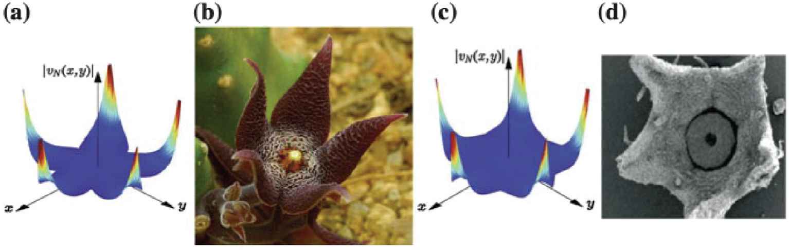
(a,c) Spatial distribution of the partial sum of order N approximating the solution of the interior Dirichlet problem for the Helmholtz equation in the flower-shaped domains with different degrees of fusion. (b) Flowers of Stapelia arenosa. (d) Nectar disc of Hekistocarpa (Rubiaceae) [58].
P8 is the principle related to optimal shapes and optimization problems. The nearly universal principle in the natural sciences is that the equilibrium configuration of a system can be found by minimizing its total energy among all admissible configurations. When considering the surface interface between two or more immiscible materials, the surface geometry is determined by minimizing the surface tension subject to whatever additional constraints are imposed by the environment. In physics, one thinks of soap films, but nature has been much more inventive. Two examples are given, one on snowflakes and one on starfish.
Concerning optimal shapes, CMC surfaces have been generalized to CAMC, constant anisotropic mean curvature surfaces [62,63]. In CMC the stress adjustment on the surface is done by agents that can move freely across the surface, for example, soap molecules in soap films. In crystals, however, the structure prevents atoms from moving in certain directions.
To define anisotropic analogs of CMC surfaces, a Wulff shape is the sphere for the “anisotropic energy” in the sense that it is the minimizer for the energy for a fixed volume. Wulff shapes can be cubes or hexagonal prisms or superellipsoids, instead of spheres (as in the case of soap). The resulting minimal surfaces and surfaces of evenly distributed stresses then have a very different shapes. The corresponding catenoid based on a hexagonal prism is shown in Fig. 4, right. The supercatenoid has the property that sufficiently small pieces of it minimize the anisotropic energy defined by the Wulff shapes, among all surfaces having the same boundary [62].
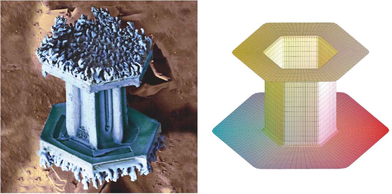
Capped column snowflake (left) and supercatenoid.
One can compare this with capped-columnar snowflakes, types that also exist in nature (Fig. 4). In this case, the corresponding minimal surface retains the hexagonal symmetry of ice molecules. Capped-column snowflakes are very different from the classic archetypical six-pointed dendritic types, but they are formed under certain conditions of temperature and humidity. One can find many other types of snowflakes like plates, needles, hollow and solid prisms, and irregular ones [12]. They may now be studied as equilibrium shapes, as zero-anisotropic stress surfaces, in analogy with soap films.
Another example of archetypical shapes is starfish, which are also a successful group of animals with an optimal form for the environments in which they live. Nature has run many experiments, however. One can find almost spherical cushion starfish with pentagonal cross-section (Fig. 5), and almost flat pentagonal shapes (cookie starfish, Fig. 6)[13].
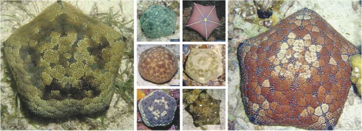
Culcita novaeguineae.
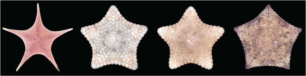
Stellaster equestris (left) and Tosia sp. (Cookie starfish).
In the case of cushion starfish (the genus Culcita, mainly found in the Philippines, Fig. 5) one may consider this as an experiment run by nature with a solution for optimal surfaces or body in between a soap bubble and an archetypical starfish (Fig. 6, left). Cookie starfish (Tosia sp.) are smaller but almost flat. Natural shapes are the result of evolutionary and developmental processes integrating a wide variety of internal and external influences.
P9: GT also led to fast computational algorithms in antenna design [46] and acoustics [52], among others. It is interesting to see how nature “computes” shape and optimization. Lamé curves and GT are non-linear, but if one considers the formation of a tree ring [9] or a square bamboo culm [10] as the result of both evolutionary and developmental processes, dealing with biotic (insects, fungi, viruses) and abiotic (light, temperature, rainfall, soil, frost, …) influences and stresses at very different time scales, it is at least remarkable that the resulting shapes are described by superellipses with exponent n ≠ 2 but not too different from 2. The formation of tree rings builds on the tree ring of previous years, incorporating all influences of the current year, to prepare for the next years. Trees convert a multi-objective optimization problem involving n-dimensional volumes, into a conservation law in two dimensions (this is Eq. (1)). This provides a completely new perspective on form and function, in many cases directly opposite to current views.
5. REFLECTIONS ON THE STATE OF THE NATURAL SCIENCES
5.1. Unit Circles and Continuity
A unified description of natural phenomena is the basis of the Scientific Revolution. Therefore, the search for unifying descriptions of a more general nature is important for scientific progress. As a generalization of the Euclidean circle, one can consider all forms described by Eq. (1) as unit circles in their own measure or metric and with their internal symmetry, in contrast to the multitude of methods in the natural sciences based on isotropy, which is the same in all directions and based on circles and spheres. In his book Minkowski Geometry, A.C. Thompson writes [64]: “Space to Euclid and Newton was uniform and “isotropic”, the same in all directions. Such a notion flies in the face of daily experience, where the connotation of up and down is different from that of east to west. There are preferred directions. Another good example is the preferred directions that cause crystals to grow as polyhedra and not spherically like soap bubbles. Unit circles and spheres are not the familiar round objects from Euclidean geometry, but are some other convex shape, called the unit ball.”
Richard Feynman wrote: “We have in our mind a tendency to accept symmetry as some kind of perfection. In fact, it is the old idea of the Greeks that circles were perfect and it was rather horrible to believe that planetary orbits were not circles, but only nearly circles. The difference between being a circle and being nearly a circle is not a small difference; it is a fundamental change so far as the mind is concerned. There is a sign of perfection and symmetry in the circle that is no longer there the moment the circle is slightly off. That is the end of it; it is no longer symmetrical. Then the question is why it is only nearly a circle – that is a much more difficult question.... So, our problem is to explain where symmetry comes from. Why is nature so nearly symmetrical? No one has any idea why” [65].
The problem seems to exist only in our minds. Supercircles |x|n + |y|n = Rn with n = 1.9999567 or n = 2.00567 are unit circles, with the classic Euclidean circle for n = 2. If we can define unit circles and coordinate systems best suited to the shape or phenomenon under study, the internal symmetry is as perfect as the symmetry of the circle. In the spirit of Lamé, the classical coordinate systems (spherical, cylindrical, even toroidal) are generalized and can be continuously transformed into any of the other coordinate systems. GT provides one-to-one transformations from one shape to one coordinate system and back.
In a discrete world it should be stressed that GT are continuous transformations. Having anisotropy in one direction, creating polarity, is essential in the evolution of life [66]. In eggs in one plane the polarity induced by selecting m = 1 in Eq. (3), generates a mirror symmetry in one direction and asymmetry (up-down) in the other. In three dimensions, avian eggs are a rotation around a central axis of symmetry defined by the asymmetry. Other solutions are found in algae, where spherical, ellipsoids and cylindrical shapes are observed [67].
5.2. From the Qualitative to the Quantitative (but not all the way)
The mathematical description brings the shape and geometry of natural shapes into the realm of the quantitative. With the equation also come the characteristic formulae to compute length, area and moment of inertia. Terms like ovoid or pear-shaped loose their meaning when a geometric transformation can turn one type into the other. “Elliptical” is a common term for the shape of many leaves in botany, but most are not elliptical at all, but superelliptical [68]. In the case of bamboo leaves, terms such as lanceolate or linear also lose their meaning when shapes can be perfectly quantified by two parameters, one for size and one for shape [69,70]. The variety of shapes in diatoms can also be unified via Eq. (3) (Fig. 7)[14,71].
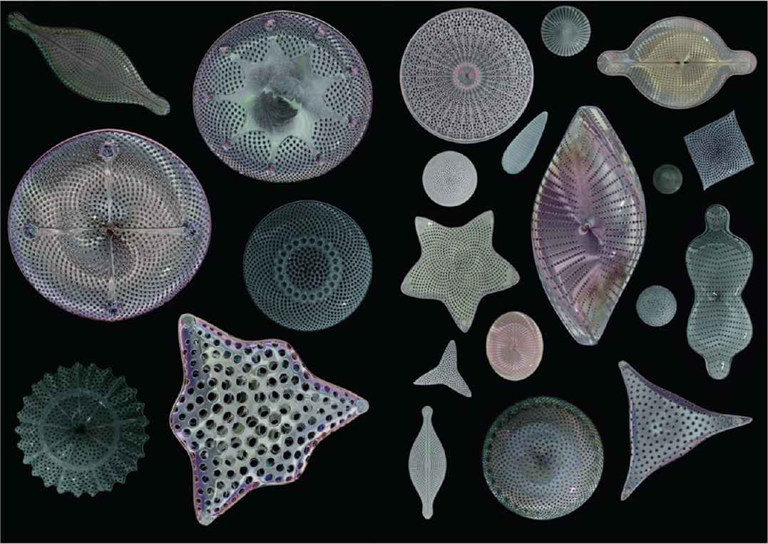
Digital diatoms [71] Courtesy of Max Seeger.
To quantify the area of eggs or leaves, one does not need any shape equation; for leaves, simple measurements of L and W are sufficient. One can use the Montgomery equation, which is a rectangle Wmax × Lmax multiplied by a constant that indicates how much of the rectangle is occupied by the area of the leaf [72] or the egg. The question then arises whether dimensions such as L and W of eggs are important for (practical or universal) formulas when modern techniques in image processing, robotics, and machine learning can use fitting methods without prior knowledge. Shape properties such as perimeter, area, moment of inertia, or curvature can then be calculated directly using the appropriate mathematical formula or recipe (e.g., number of pixels).
On the other hand, striving towards a complete quantification of phenomena would be a tragic mistake. The work of Henri Poincaré (1854–1912) in this field is of lasting importance. Richard Feynman wrote [65]: “The next great era of awakening of human intellect may well produce a method of understanding the qualitative content of equations. … Today we cannot see whether Schrödinger’s equation contains frogs, musical composers, or morality – or whether it does not. We cannot say whether something beyond it like God is needed, or not. And so, we can all hold strong opinions either way”.
6. CONIC SECTIONS AT THE CORE, ONCE MORE
6.1. Universal Natural Shapes
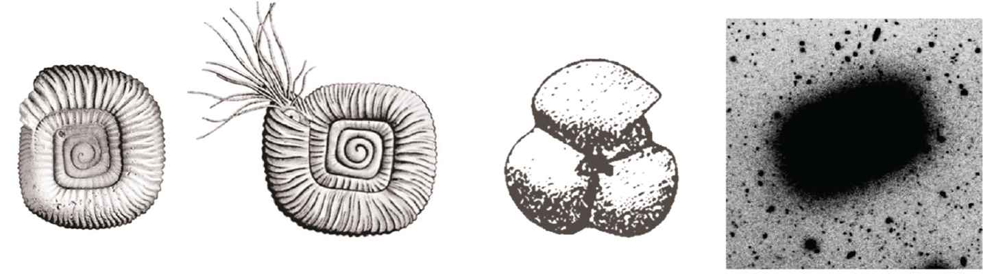
GT checks all the principles, and work is ongoing to determine how universal it is. In general, application of the corresponding Gielis transformations to the “most natural” curves and surfaces of Euclidean geometry (for dimension 2: the circles and the logarithmic spirals), results in many of the forms that we do observe in nature, in biology, crystallography, physics and chemistry [8]. So far we have focused on transformations of the circle (or constant functions), but there are multiple examples with spirals, in mollusk shells [73,74] and ammonoids. In various groups of ammonoids triangular [75,76], and quadrangular coiling [77], has been reported (Fig. 8). The universe itself provides examples of superelliptical galaxies (Fig. 8) [78,79].
On the theoretical side, properties of GT have been studied in [80,81]. They can describe regular polygons [57]or regular polygons with alternating long and short sides or edges, when A ≠ B in Eq. (3). Unsurprisingly – at least with knowledge of GT – one finds such shapes in silver halide crystals (Fig. 9), and in triangular snowflakes. But whereas in our modern times one would recognize a truncated triangle, where symmetry breaking from six to three is necessary, with GT it is a hexagon with alternating short and long sides, in the same way a rectangle is related to the square. Within the framework of GT, this shape preserves the hexagonal symmetry of ice and silverhalide. No symmetry-breaking of any kind needs to be invoked, nor are extra assumptions or hypotheses required.
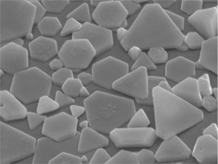
Silver halide crystals, all hexagonal, either with the same side length or with alternating long and short sides.
GT provides a new set of glasses or lenses, allowing us to adjust our perception of natural shapes and phenomena, as variations of a single principle, as examples of a continuum, also in geometry and mathematics. The Lorentz-Fitzgerald transformations of Special Relativity Theory are a special case, and the origin of elliptic functions reveals the same mathematical structure. Moreover, our relativistic space-time universe itself is also described by similar formulae (Friedman-Lemaître-Robertson-Walker) [8]. They are all examples of the simplest Minkowski geometry (Eq. (5a), [61]) [64], and the simplest Riemann-Finsler metrics (Eq. (5b)) [57]:
In his famous Habilitationsschrift, B. Riemann (1826–1866) had already mentioned the geometric tangent 2D-indicatrix
Peter L. Antonelli (1941–2020) wrote [82]: “As is well known, Riemann foresaw the advent of Finsler geometry (the 1918 thesis of P. Finsler, a student of Carathéodory) when he gave an example of a line-element defined as the 4th root of the sum of 4th powers of the independent coordinate increments, which contrasted sharply with the familiar Pythagorean expression. Nevertheless, if there were no scientifically useful examples, Riemann’s cursory remarks would hardly constitute reason for a scientific study”. Since the 1990’s we have many, many examples from biology and other fields in the natural sciences. GT are used in the geometry of wave propagation in seismic phenomena [83]. Meanwhile, GT have already won their place in the history of geometry and mathematics [84].
6.2. Allometry and Parabola’s
Using the two main mathematical operations, addition and multiplication, the Universality-Unification principle P6 suddenly becomes very clear.
Superellipses result when two variables x, y raised to powers n and m are added. When, but if they are multiplied (xn × ym), or compared (xn/ym). As a result, one obtains all the power laws as superparabolas (Table 1). Both power laws and superellipses are examples of conservation of area (in this case n-area).
| Variables x, y | Addition | Product |
|---|---|---|
| Exponents n, m | ||
| Result | xn + ym |x|n +|y|m |
ym = xn y = xn/m |
| Means | Arithmetic means | Geometric means |
| Curves | Lamé curves Superellipses |
Superparabolas Power laws |
| Effect | Shape and size | Allometry |
Lamé curves and superparabolas.
Power laws are ubiquitous in the natural sciences. Hence, large numbers of phenomena in the natural sciences can be encompassed in a single framework, namely a generalization of conic sections. The planar graphs or curves, super-versions of the classic conic sections, are then two-dimensional conservation laws, based on n-dimensional volumes (a sum or product of n or m-dimensional cubes), where the dimensions need not be integer. In the same way, as supercircles are generalizations of circles, these power relations are superparabola’s, generalizations of the classic parabola y = x2.
In Fig. 10 left superparabola’s ym = xn are shown in the interval [0;1], with the exponents ranging from n = 1/2 to n = 2 with steps of 1/5. The cases for n > 1 and n < 1 have y = x with n = 1 as the symmetry axis (the bisectrix). A classic parabola is a machine that turns a rectangle with an area 1 × y into a square with the same area, and side x. In the same way a superparabola ym = xn turns a beam with an n-volume into a cube with an m-volume (for n < m). All power laws have simple graphical expressions. They are most often represented as straight lines, using logarithmic transformations.
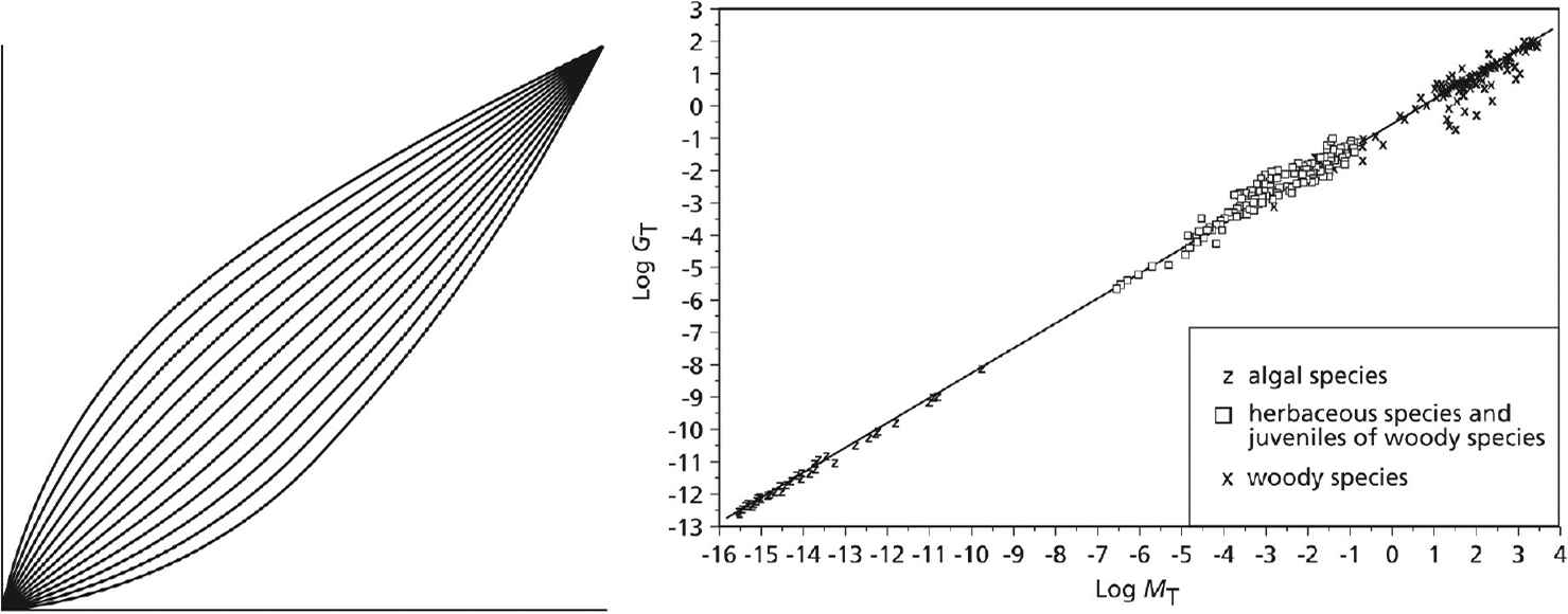
Left: sub- and superparabolas in the interval [0;1]; Right: Metabolism MT versus biomass GT from smallest plants to the largest trees [85].
Fig. 10 right shows the allometric relationships between biomass and metabolism in plants over a wide range of plant sizes, from small algae to the largest trees. Fig. 11 displays such relationships in planets, codified in Kepler’s Law.
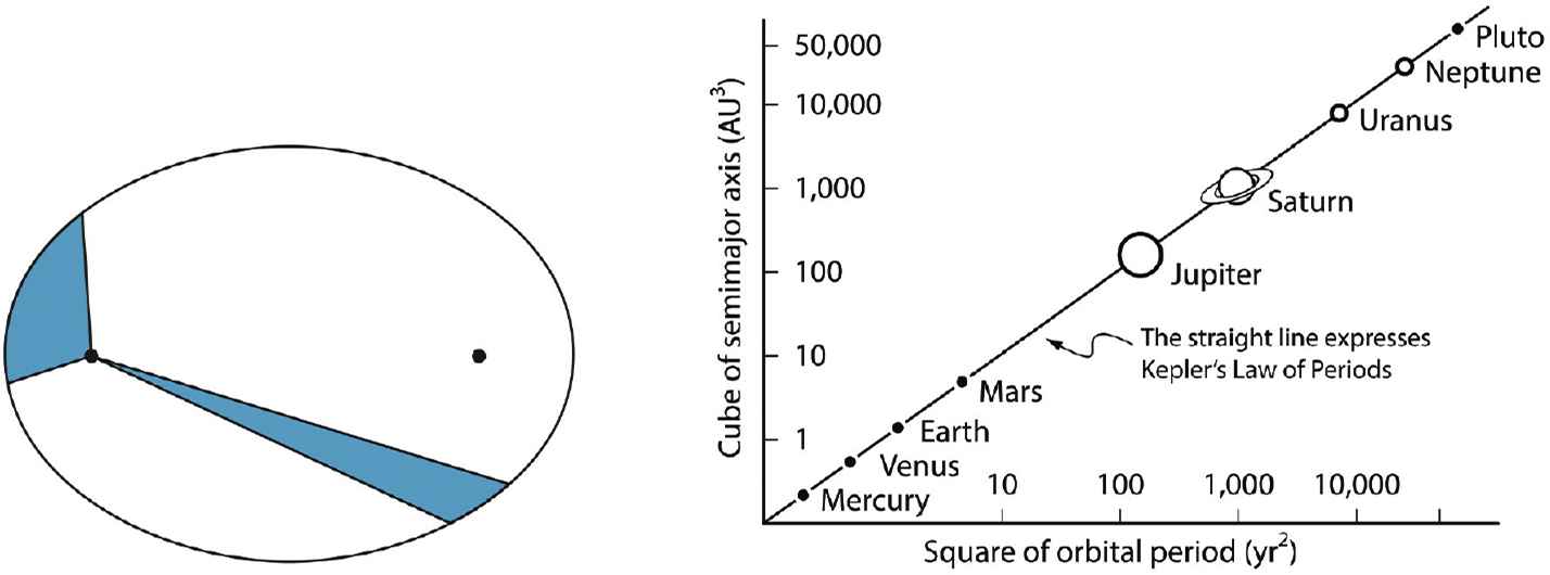
Kepler’s Law of Equal Areas in equal times (left) and his law on the square of orbital period versus the cube of the semi-major axes of the elliptic orbit (right) [12].
6.3. Allometry: A Theory of Everything?
Allometric laws are called laws because they do the same as the laws of physics, namely reducing complex relationships to simple relations between two measurable quantities. The relation between metabolism and size is shown in Fig. 10, as one example. These relations may be linear, or the quantities may be raised to some power (e.g. in Kepler’s Law of Equal Areas, Fig. 11). All laws of physics fit in this framework as well.
K.J. Niklas investigated the state of the art [85]: “The importance of the study of allometry extends beyond description or prediction. If certain trends are size-dependent and ‘invariant’ with regard to phyletic affinity or habitat, they draw sharp attention to the existence of properties that are rooted in all, or at least, most living things. Identifying these properties using a first principles approach, therefore, has become something of a Holy Grail in biological allometry because any successful theory would unify as many diverse phenomena in biology as Einstein’s general theory of relativity has for physics”.
He concludes [85]: “These comparisons provide strong statistical support for each of the allometric predictions. This support is taken as evidence that a general unifying allometric theory for plant biology is near at hand. Nevertheless, the validation of this theory requires much additional work and raises a number of procedural and conceptual concerns that must be resolved before a single ‘global’ theory is accepted”.
From a geometrical perspective, if allometry is thought of as a collection of straight lines obtained by least squares fitting of pairs of data points on morphology, physiology, or ecology for individuals, or populations, with a single regression line for each data pair, then allometry becomes a sort of species-specific blue-print of internal architecture, or of external architecture as observed in plant phyllotaxis, the forms of flowers or in seashells (e.g. [86]). Finsler geometry plays a crucial role [87], and “one important finding in Finsler science is the equivalency to Hilbert’s 4th problem, that of classifying the Finsler geometries having straight lines as shortest distances between two points, where straight lines are allometries holding globally” [86]. Finsler geometry is also directly related to Hilbert’s 23rd problem on the calculus of variations [88].
6.4. Only Half the Story
Power laws are found everywhere, as well, from the size of cities to the power noise in time series, but superelliptical structures are also found everywhere, in physics, chemistry, biology, and even in the economy [89,90].
A prime example of allometry in economy is the Cobb-Douglas production function, with the certain exponent, depending on the substitution parameter δ. This is equivalent to an expression like z = xn · ym. In the case of Cobb-Douglas n = 1 − m. The Cobb-Douglas model is a limiting case of the CES (constant elasticity substitution) production models (in the case of δ = 0 elasticity reduces to unity) [89]:
Lamé’s footprint is everywhere. Despite different appearances it all fits into one coherent framework, of generalized conic sections (Table 1, [12]). In the framework of conic sections, we can safely say that power laws are only half of the story. Moreover, the general unifying allometric theory for plant biology should also adhere to the nine principles. They do check P1-3 and P4-6, and by integrating this allometric theory of biology into the broader geometrical framework described above, also P7-9, many more shapes and phenomena can be unified.
Still, we are only one step beyond the conic sections of Apollonius, Kepler, Galilei, and Descartes. By extending conic sections with power laws and GT, starfish, flowers, leaves, eggs, tree rings, and superelliptical galaxies are all comparable or commensurable. They provide a universal framework for geometrically describing a very wide range of natural shapes at all scales, treating both population-level and ensemble-levels in general, and describing individual differences with arbitrary precision, as a complete scientific methodology.
7. CONCLUSION
7.1. Nine Principles
There are numerous ways of applying mathematics in the natural sciences. But if we assume that a further development in the Scientific Revolution is possible, it will involve the two phases, the Keplerian and the Newtonian phase (R. May distinguished three phases, named after Tycho Brahe (1546–1601), Kepler and Newton: observed facts, patterns that give coherence to the observations, fundamental laws that explain the patterns [92]). A unified description should then be in the spirit and tradition of the ancient Greek mathematicians, and it must be tested against each of the nine principles, not only to understand the potential but also to establish its limitations and its limits.
Three groups were defined, with three principles each. The first group focuses on the complexity of the model, with single curves and topologically simple. This follows another scientific tradition, namely that many solutions to problems in physics and biology are found to be a limited number of curves (conic sections, catenary, cardioid, ...).
The second and third group build a bridge between mathematics and the real, observable world. The second group focusses on how well the models fit the data. This group is crucial to establish a given model as a scientific method, but at the same time it explores how widely applicable a uniform description is. Obviously, this Universality Principle is open ended, or unbounded. The third set of principles relates to mathematical physics and to what extent the uniform description allows us to understand the why and how of natural shapes, forms and phenomena.
It was shown how developments including allometry, superellipses and Gielis Transformations, comply with the nine principles. These principles provide a standard for universal equations in the context of the scientific revolution, and in this context, the NRG equation for eggs has only limited validity. Compliance with these principles is only a start; a huge amount of theoretical and practical work is needed, in cooperation with experts in various fields of science.
7.2. Geometry at the Core, Once More
We stressed the importance of the first set of principles (P1-P3). The full statement of V.I. Arnold on complex models is [27]: “Complex models are rarely useful (unless for those writing their dissertations). The mathematical technique of modeling consists of ignoring this trouble and speaking about your deductive model in such a way as if it coincided with reality. The fact that this path, which is obviously incorrect from the point of view of natural science, often leads to useful results in physics is called “the inconceivable effectiveness of mathematics in natural sciences” (or “the Wigner principle”). Here we can add a remark by I.M. Gel’fand: there exists yet another phenomenon which is comparable in its inconceivability with the inconceivable effectiveness of mathematics in physics noted by Wigner – this is the equally inconceivable ineffectiveness of mathematics in biology.”
Geometry provides a new perspective. GT are a simple generalization of circle, ellipse, and the other conic sections, which formed the foundation of the Kepler-Newton model of science [92] for all the great successes of science up to the present day, especially for the great and the small. It began with Kepler’s step of unifying descriptions of certain phenomena and culminated in Newton’s laws of motion guiding those phenomena (without the need for hypotheses of any kind), with analysis as the toolbox.
The first step in this program is a unifying description of shapes and phenomena, using allometry and Lamé’s superellipses. The full title of [8]is: Universal Natural Shapes: from the supereggs of Piet Hein to the cosmic egg of Georges Lemaître. Supereggs, avian eggs and the cosmic egg, the mathematical basis of the Big Bang, are now captured in one framework, along with all the power laws, ubiquitous in biology and science. We showed that these are all simple extensions of the very classic conic sections and the application of areas, known to the Pythagoreans, but with very clear contemporary links in geometry and mathematics.
The geometrization of the natural world, including the living, is far from complete [1]; we only are taking the first steps. We provide a method of investigation of the natural world, not a final theory or law. Like Galilei’s telescope and Hooke’s and Van Leeuwenhoek’s microscopes, it allows us to see the unseen, and opens the door to new discoveries. Moreover, we should never forget that science, including all physics, are only models and approximations of reality. However, it provides for a coherent framework to look at objects, phenomena and dynamical systems from a uniform and unified perspective, ensuring that eggs, starfish, flowers and many, many more shapes, objects and phenomena, become commensurable. In his On the Origin of Species [93], Darwin wrote: “There is grandeur in this view of life, ..., from so simple a beginning endless forms most beautiful and most wonderful have been, and are being, evolved”. In this case, the so-simple-a-beginning is the conic sections, with parabola for precise fitting, and hyperbola and ellipse for too much and too little, known to the Pythagoreans.
Conflict of Interest
The authors declare no conflicts of interest. Note that because the first and corresponding author of this article is the Editor-in-Chief of the journal, the peer review process has been managed independently from the Editor-in-Chief by appointing a separate Handling Editor to oversee the process and make the final decision.
Authors Contribution
J.G., P.S. and D.C.: conceptualization; J.G.: writing the original draft of the manuscript; J.G., P.S. and D.C.: review & editing of final manuscript.
Funding
The authors declare no funding.
Data Availability
The experimental data that support the findings of this study are openly available in references [9–13,34,37–52,63,68–70 (and references therein)].
Acknowledgments
The authors like to express their gratitude to the handling editor and the reviewers
REFERENCES
Cite This Article
TY  - JOUR
AU  - Johan Gielis
AU  - Peijian Shi
AU  - Diego Caratelli
PY  - 2022
DA  - 2022/08/17
TI  - Universal Equations – A Fresh Perspective
JO  - Growth and Form
SP  - 27
EP  - 44
VL  - 3
IS  - 1-2
SN  - 2589-8426
UR  - https://doi.org/10.55060/j.gandf.220817.001
DO  - https://doi.org/10.55060/j.gandf.220817.001
ID  - Gielis2022
ER  -


