
Additional information: Department of Mathematics, University of the Basque Country, Bilbao, Bizkaia 48060, Spain
Accepted 2 December 2019
Available Online 2 March 2020
- DOI
- https://doi.org/10.2991/gaf.k.200124.003
- Keywords
- Anisotropic
elastica
lemniscate - Abstract
We classify the anisotropic elastic curves modulo rescaling and quasi-rotation depending on one parameter for an ample family of anisotropic functionals. Several illustrations of this classification are shown at the end.
- Copyright
- © 2020 The Authors. Published by Atlantis Press SARL.
- Open Access
- This is an open access article distributed under the CC BY-NC 4.0 license (http://creativecommons.org/licenses/by-nc/4.0/).
1. INTRODUCTION
Instances of one-dimensional continua having geometries determined by minimization of a bending energy are ubiquitous in the mathematical, physical and biological sciences. These range from models of elongated beams used in construction to the flagella of microorganisms. In our everyday experience, we encounter a myriad of fibers, wires, cables, hoses and rods whose shapes are determined by this type of variational principle. One commonly encountered aspect in the study of these continua, which we henceforth refer to as rods, is that the governing energy may be anisotropic, i.e. it is dependent on the direction of the curve, as represented by the unit tangent vector T. Understanding the morphology of rods is essential since the geometry is a visual manifestation of the physical properties acting on the rod.
In a recent paper [1], we developed a methodology to study the equilibria arising from minimizing a specific type of anisotropic bending energy in two and three dimensions. In this model, the Young’s modulus, which measures the rod’s resistance to bending, is given by a continuous periodic function of the angle the tangent makes with a fixed direction. In the two dimensional case, the equations for the extremals of this bending energy are easily integrated and all examples can be explicitly found. We recall that in the isotropic case, this is usually achieved via elliptic functions but our method does not rely on this tool.
In the isotropic case, the problem of determining the bending deformations of rods was first formulated by J. Bernoulli in 1691. Later, D. Bernoulli, in a letter to L. Euler, suggested to study elasticae as minimizers of the bending energy. Then, L. Euler [2] (see also the translation [3]) achieved a classification of planar elasticae into nine specific types, although some partial results were already known to J. Bernoulli. For more details about the history of (isotropic) elasticae we refer to [1] and references therein.
How is Euler’s classification affected if the rod’s energy is anisotropic? This is the principal question we consider. The main result of the present paper is to show that for functionals possessing an essential symmetry, all of the types in Euler’s classification are present although the order in which they occur, in terms of a governing parameter, may be more complicated than in the isotropic case. Also, in the anisotropic case, there is an additional degree of freedom arising from quasi-rotations of each of the nine types.
The paper is organized as follows. In Section 2 we describe the materials and methods used for the development of the paper. In Section 3.1, we formulate the definition of anisotropic elasticae and discuss their properties. In particular, the representation formula is presented. Section 3.2 is devoted to the classification of anisotropic elasticae into nine different types. Then, in Section 3.3, we illustrate this classification for several choices of Wulff shapes. We finish with some conclusions in Section 4.
2. MATERIALS AND METHODS
As mentioned earlier, Euler’s classification of isotropic elasticae relied heavily on the use of elliptic functions in order to represent his elasticae. In the anisotropic case, this tool is no longer applicable however we had previously found a relevant representation formula which can be applied to represent the curves. Since our classification theory is centered around a particular type of curve, the lemniscate, it was necessary to prove its existence. Because of the generality in the type of functional we consider, these curves could not be parameterized exactly. Instead, we rely on standard techniques of mathematical analysis to prove their existence.
Constantly, while conducting this research, it was necessary to employ computer graphics in order to generate hypotheses about how the classification would proceed and to test them. Both the Maple and Mathematica softwares were used for this purpose in an essential way. This went substantially beyond there use to generate the graphics displayed in the article.
3. RESULTS
3.1. Anisotropic Elasticae
Let γ: S1 → R+ denote a sufficiently smooth function satisfying the following convexity condition. We require that if θ denotes the usual polar angle in the plane, then
For purposes that will be clear later, we introduce the curve Ω⊥ which is a clockwise rotation of Ω through an angle π/2.
For any smooth, regular (planar) curve C: I → R2, we denote by T its unit tangent and by N its unit normal with N = JT where J is counter-clockwise rotation by an angle π/2. We represent T by eiθ and write γ(θ) as γ(T) when desired. If κ denotes the curvature of C, then the anisotropic curvature is defined by
As in [1], we define the anisotropic bending energy of C by
Regardless of the boundary conditions, any equilibrium curve of ℰβ must satisfy its associated Euler–Lagrange equation. We will refer to such a curve as an anisotropic elastic curve for the energy density γ. Critical points of ℰβ, i.e. anisotropic elastic curves, are characterized in [1] by the conservation law
On the other hand, if p ≠ 0, a representation formula for planar anisotropic elasticae was obtained in [1] [see formula (10)]
If we differentiate (5) with respect to θ, we see that eiθ is the unit tangent map of the curve into S1. Clearly, θ is restricted by
Notice that, after rescaling if necessary, the constant of integration p in (4) and (5), may be assumed to be p = 1/2, as the following proposition shows.
Proposition 1.
Let C be a critical curve of ℰβ. Then, any rescaling of ratio r > 0,
Proof.
Let C be a critical curve of ℰβ for p ≠ 0, then the anisotropic curvature of C, λ, verifies the conservation law (4).
Now, if we apply a rescaling of ratio r > 0 to C, say
Thus, substituting this in (4) we obtain
Moreover, if we apply a change of variable
This expression represents a quasi-rotation of an anisotropic planar elastica with θ0 = 0. In fact, if we rotate the Wulff shape Ω by the replacement γ(θ) → γ(θ – θ0), then the expression (7) above is just the rotation of an anisotropic planar elastic curve for the rotated Wulff shape. The parameter θ0 induces a transformation of the elasticae which is insignificant in the isotropic case.
3.2. Classification Results
In this section, we will classify planar anisotropic elasticae modulo rescaling and quasi-rotation for symmetric Wulff shapes. Therefore, as mentioned above, we can assume that p = 1/2 and θ0 = 0, so that the representation formula for anisotropic planar elasticae (5) now reads
The constant β is restricted by β > −1. For these values of β, there may be isolated points where (see [1])
At these points, the curvature of C, κ, also vanishes and, therefore, they represent inflection points of the curve C(s).
A particular type of lemniscate appears in Euler’s classification of isotropic elastic curves given in [2]. This curve is the only closed elastica with non-constant curvature.
We begin our classification by proving the existence of an anisotropic analogue for this curve in the case that the functional possesses a symmetric Wulff shape. These examples appear whenever the inflection points of C(s) happen to be double points. In the anisotropic case, however, this lemniscate may not be unique. An example is given below of a functional having three distinct anisotropic lemniscates.
We will need the following technical lemma.
Lemma 1.
Let μ be any positive function. Then, the function
Proof.
We begin by proving that the function
Consider the limit of the third integral, I3, when
For the second integral, I2, we make the change of variable θ = π/2 + ω + t to obtain
Moreover, a similar argument works for the first integral I1 and, therefore,
as
Now, we just need to check that in the interval (π/2, π) there is a change of sign, so that there exists a zero of
Now take a δ > 0, such that δ < π/2, then at ω = π−δ we have
Then, taking the limit as
We deduce from this the following existence result.
Theorem 1.
For any symmetric Wulff shape Ω, there exists a constant βl ∈ (0,1) such that the critical curve of ℰβl with non-constant anisotropic curvature, λ, is closed.
Proof.
Let 0 < β < 1 and denote by C(s) any critical curve of ℰβ with non-constant anisotropic curvature. The inflection points of C(s) are given by the solutions of (9). By (6), these points are, precisely, θ = π/2 ± ω depending on the value of ω ∈(π/2, π).
As noticed above, we have that the closed critical curve appears whenever the inflection points are precisely the double points of the curve C. This means that C(π/2 + ω) = C(π/2 – ω).
Define the (a priori complex-valued) function
The result follows by checking that there exists a value ωl such that ψ(ωl) = 0, since this ωl would give rise to a value βl [see (6)] whose associated critical curve is closed.
Note that ψ takes only real values. In fact, by using the representation formula for C (8), we have that for any ω ∈ (π/2, π),
Then, it is clear that
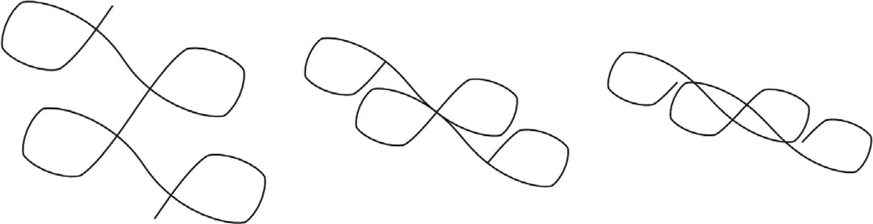
Up to quasi-rotations and rescalings there is at least one anisotropic elastica with non-constant anisotropic curvature associated to βl ∈ (0, 1) which we will refer to as an anisotropic elastic lemniscate (For some illustrations, see Figure 1).
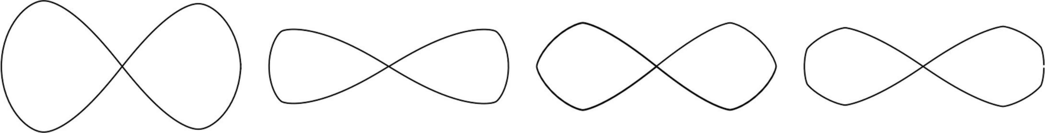
Lemniscate elasticae (0 < βl = β < 1).
Now, we are in conditions to prove the classification of planar anisotropic elasticae.
Theorem 2.
Let C be a planar anisotropic elastica for a symmetric Wulff shape Ω, i.e. a critical curve of ℰβ. If the anisotropic curvature of C, λ, is constant, then C is either a straight line (λ = 0) or a rescaling of Ω⊥ (λ2 = β).
If λ is non constant, we have the following families depending on the parameter β > –1:
- 1.
Orbit-like anisotropic elasticae, if β > 1.
- 2.
Borderline anisotropic elasticae, if β = 1.
- 3.
Wave-like anisotropic elasticae, if –1 < β < 1. In this case, we have the following sub-cases:
- (i)
Multiloop anisotropic elasticae, if 0 < β = –sin(π/2 + ω) < 1 and ψ(ω) < 0.
- (ii)
Lemniscate anisotropic elasticae, if 0 < β = βl < 1.
- (iii)
Deep waves, if 0 < β = –sin (π/2 + ω) < 1 and ψ(ω) > 0.
- (iv)
Rectangular anisotropic elasticae, if β = 0.
- (v)
Shallow waves, if –1 < β < 0.
- (i)
Proof.
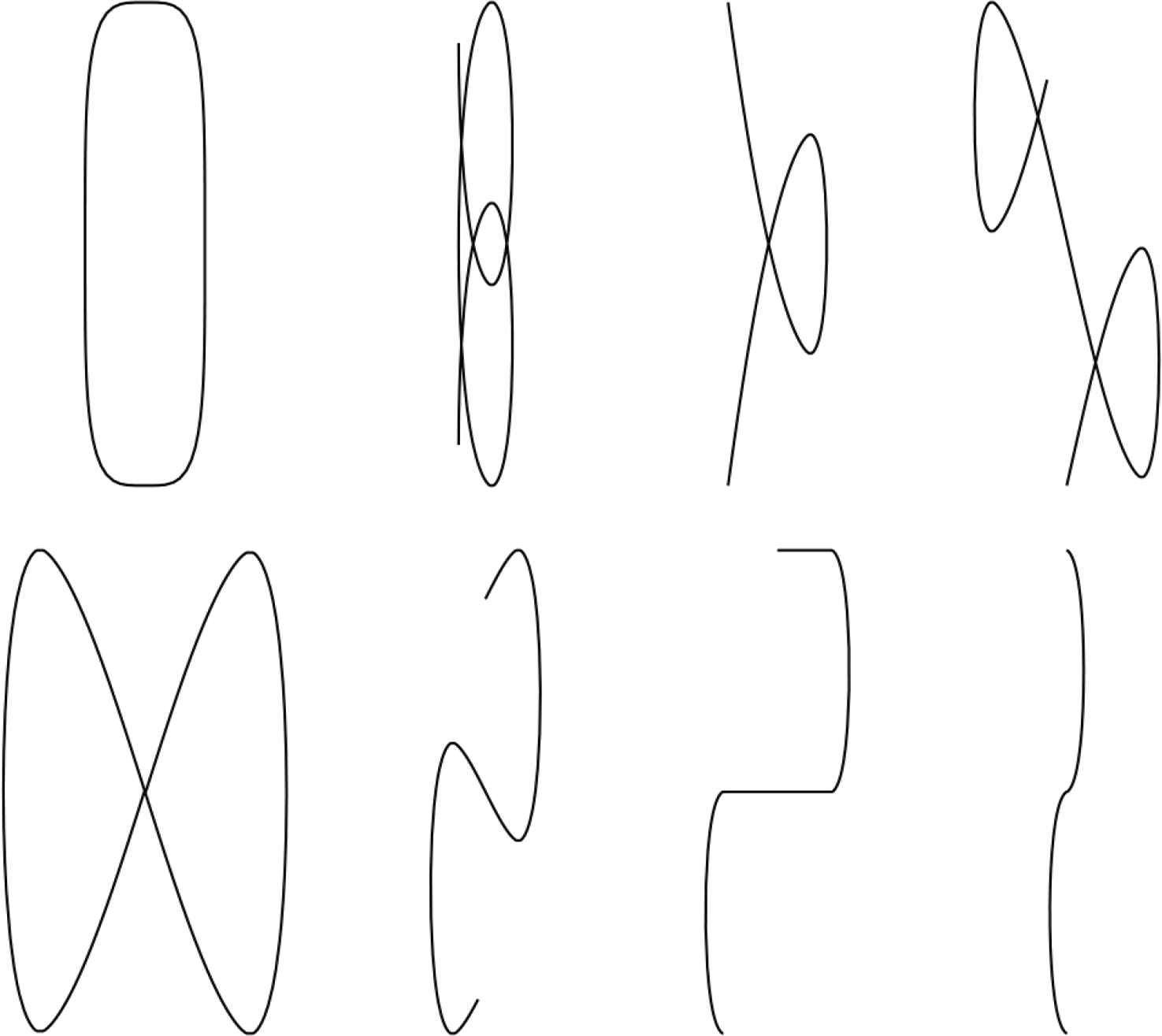
Let C be a critical curve of ℰβ for a fixed β. The case λ constant has been explained before, giving rise to either straight lines or rescalings of Ω⊥ (see Figure 2). Thus, from now on, we assume that λ is not constant. We recall that θ represents the angle that the tangent to C makes with the horizontal axis. The proof is going to be divided in terms of the different possible values for β.
The Wulff shapes Ωn, for n = 2, 3, 4 and 6. Recall that the critical points with λ2 = β correspond to 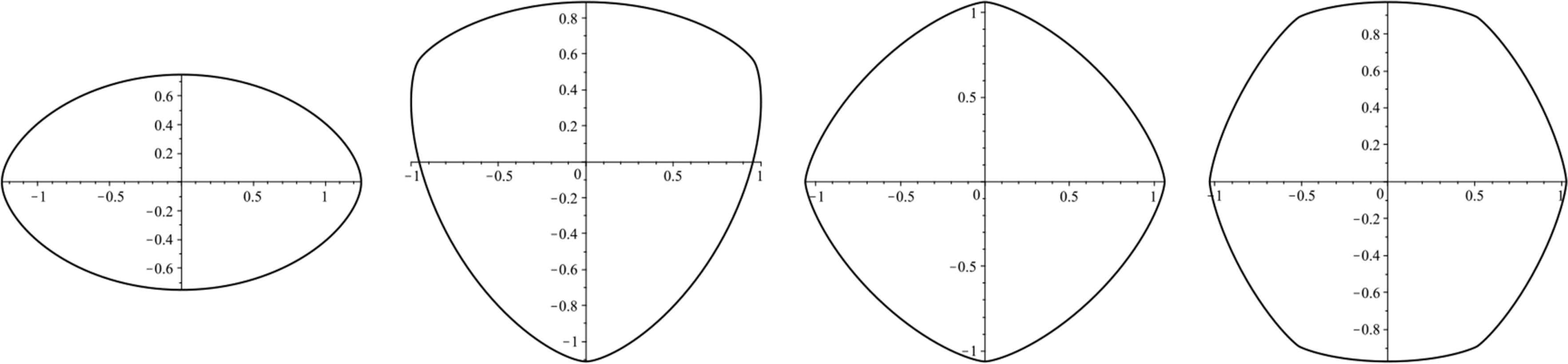
We begin by considering β > 1 (see Figure 3). In this case, (9) tells us that λ never vanishes, i.e., there are no inflection points on the anisotropic elastica C and, as a consequence, θ varies in the whole real line. Thus, we have orbit-like anisotropic elasticae.
Orbit-like anisotropic elasticae (β > 1).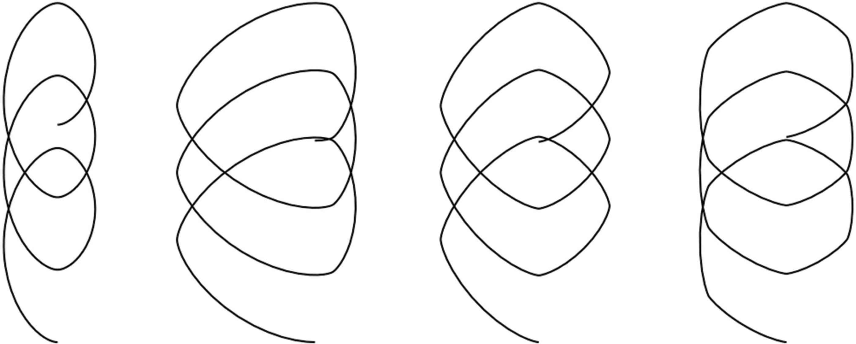
If –1 < β ≤ 1, from (9) it is clear that at any interval of length 2π where θ varies there are exactly two inflection points. Therefore, θ is only defined in an open interval of length smaller or equal 2π starting at one inflection point, and finishing at the other one. This means that if we consider our anisotropic curve C to start at one of those inflection points, θ varies until reaching the following inflection point, then, θ goes back again.
Take now β = 1 (see Figure 4). In this particular case, the domain of definition for θ can be considered to be (–π/2, 3π/2). Now, since limθ → –π/2λ = limθ →3π/2λ = 0, we have that the curve C tends to a straight line at the end points. Moreover, the tangent at the end points tends to make an angle of –π/2 (3π/2, respectively) with the horizontal axis, i.e. C tends to a vertical line. This case gives rise to a single loop and, hence, it corresponds with borderline anisotropic elasticae.
Borderline anisotropic elasticae (β = 1).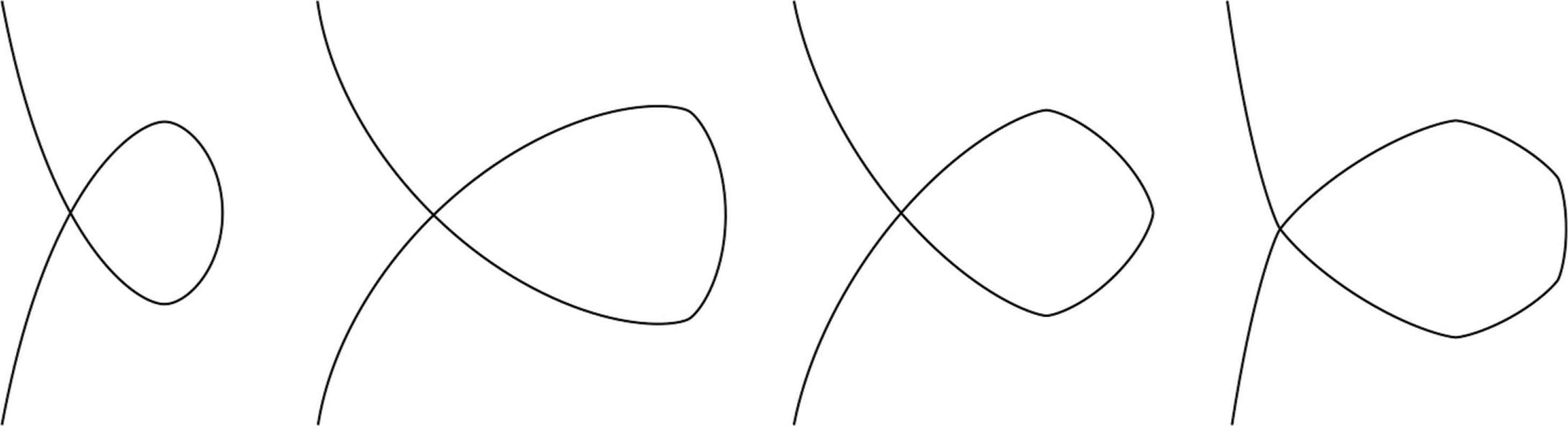
Assume 0 < β < 1. For a fixed β, we define the function
By a similar argument as in Lemma 1, we have that above function is continuous for t ∈ (0, ω). Recall that ω is defined by (6) in terms of β, hence, it is a fixed value, ω ∈ (π/2, π). The limit of
- •
Sub-case 0 < β < 1 and ψ(ω) < 0 (see Figure 5). In this case, the function
- •
- •
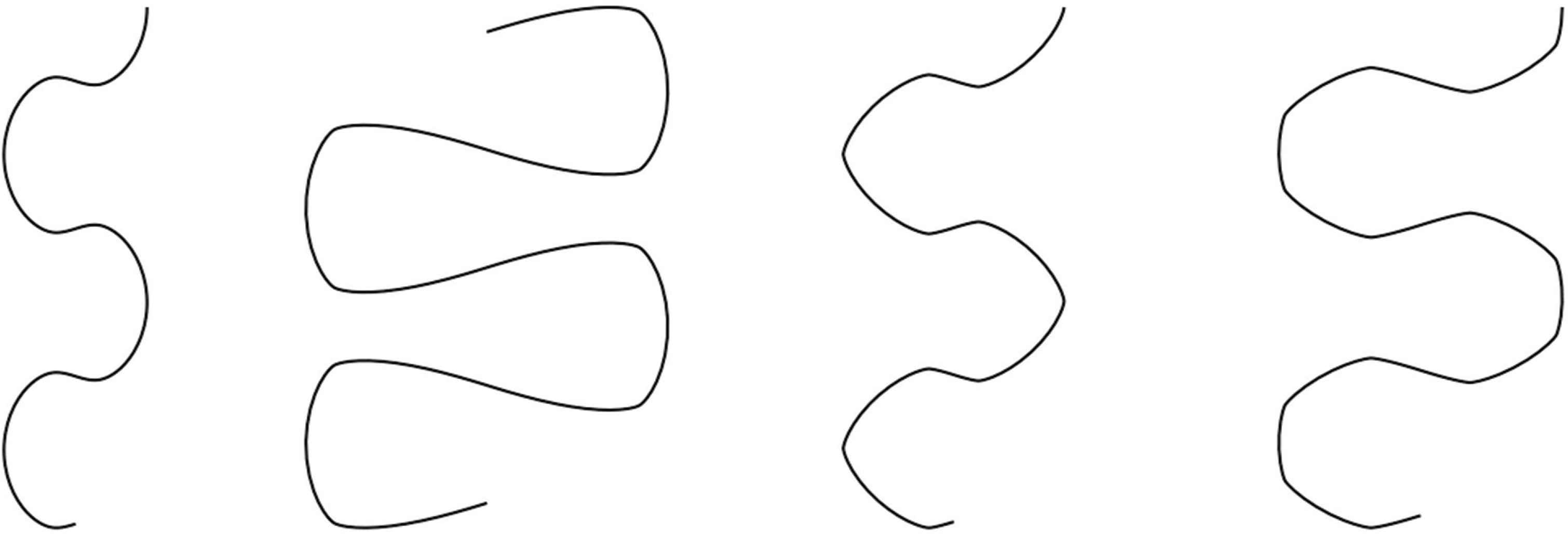
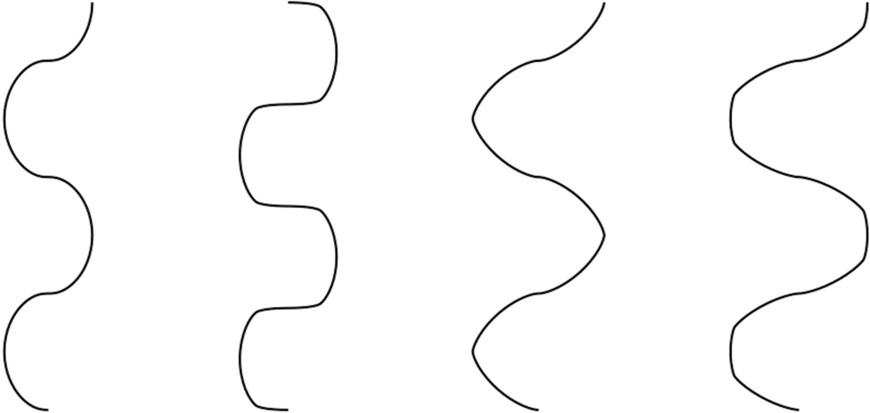
Sub-case 0 < β < 1 and ψ(ω) > 0 (see Figure 6). Contrary to the multiloop case, here, we have that
Now for β = 0 (see Figure 7), the domain of the tangent map on S1 is a semicircle, since θ ∈ (0, π). Hence, this corresponds with the rectangular anisotropic elasticae. Note that in this case, the anisotropic elastica cuts the vertical axis orthogonally.
Multiloop anisotropic elasticae (0 < β < 1 and ψ(ω) < 0). Deep waves (0 < β < 1 and ψ(ω) > 0). Rectangular anisotropic elasticae (β = 0).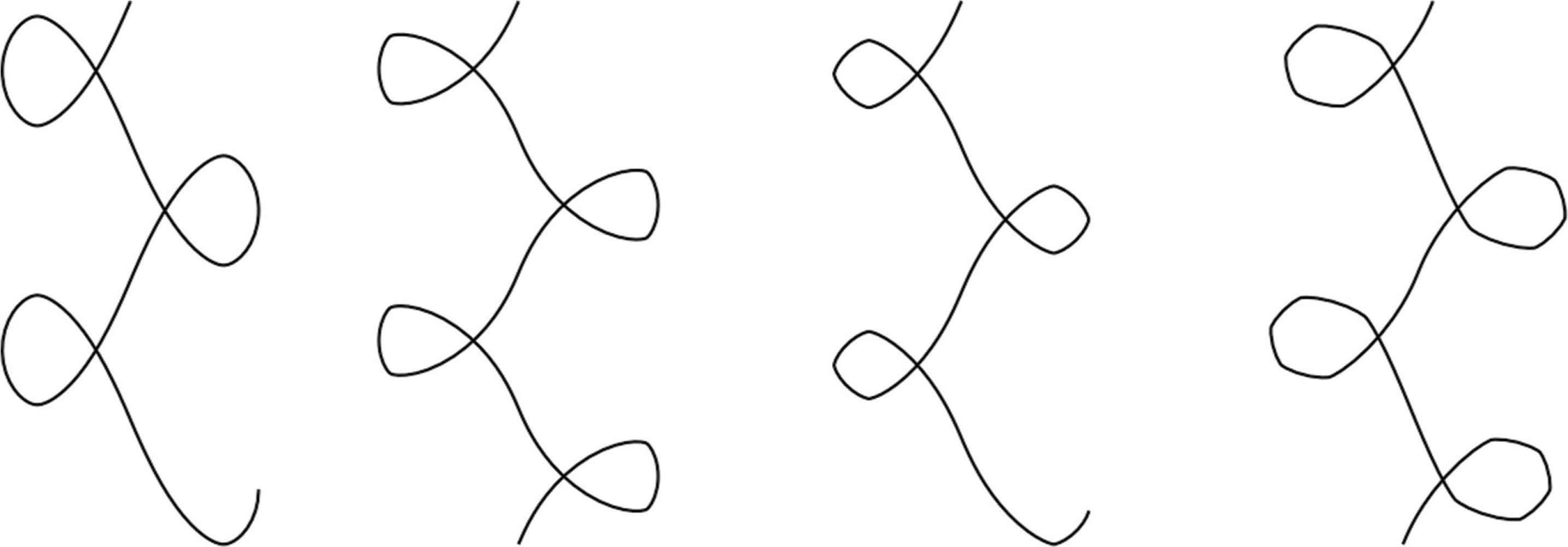
Finally, for the case –1 < β < 0 (see Figure 8), the arc-length of the domain of the tangent map is smaller than π, producing shallow waves. This finishes the proof. q.e.d.
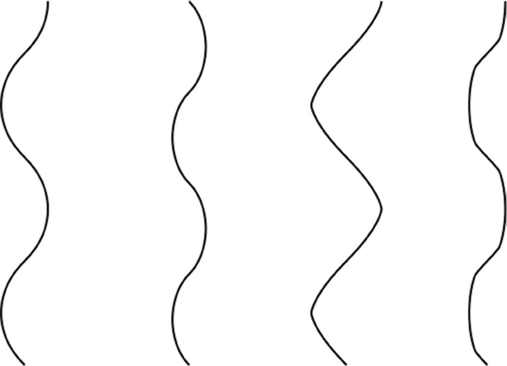
Shallow waves (– 1 < β < 0).
For many choices of γ, the types of elasticae vary ‘monotonically’ as β decreases. However for others, we observed that this is not the case due to some oscillation in the sign of ψ(ω). In particular, Figure 9 shows three distinct lemniscates which occur for the functional having density γ16:= 1 + cos(16 θ)/(16)2. The Wulff shape for this functional is a smoothed 16-gon (See Section 3.3 for more details).
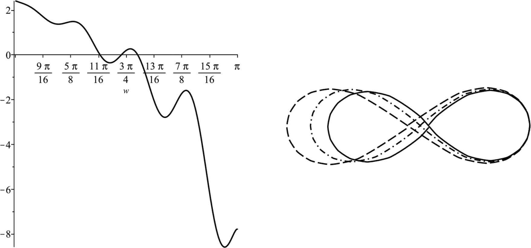
The function ψ(ω) for the density γ16 (Left); and the three distinct lemniscates (Right)
As a final remark, observe that the existence of anisotropic elastic lemniscate is not guaranteed if the Wulff shape does not verify the symmetry condition (1), since, in this case, ψ(ω) ∉ R [see (10)] and therefore the analysis made in Lemma 1 is not applicable. Indeed, consider the non-symmetric Wulff shape
Then, as suggested in Figure 10 there are no anisotropic lemniscates for this Wulff shape
Evolution of anisotropic elasticae for
3.3. Illustrations
In order to obtain some illustrations of above classification, we consider the following densities. If n is an even positive integer, we define
Then,
On the other hand, if n is an odd positive integer, γn is going to be
In these cases,
We will refer to the Wulff shape for the density γn as Ωn. The distinction between the odd and even cases is done so that the function μ verifies the symmetric condition (1). Several illustrations of these Wulff shapes and the different types of associated anisotropic elasticae, produced using (8) are shown in Figures 1–8.
To obtain a greater variety of Wulff shapes, we will use the following construction. Take the polar coordinates (r, θ), where the radial function r = r(θ) is given by
We are going to choose the following constants b = 1, a = ma = mb = na = nb = n = 4 and denote by
The rotated Wulff shape together with its associated anisotropic elasticae are shown in Figure 11. As before, these anisotropic elasticae are obtained using the integral expression (8).
Anisotropic elasticae for the Wulff Shape,
4. CONCLUSION
We have shown that, assuming the Wulff shape of the functional has the right symmetry, all types of elasticae found by Euler have an analogue in the anisotropic case. In addition, images of these curves are easily accessible via computer graphics.
CONFLICTS OF INTEREST
The authors declare they have no conflicts of interest.
ACKNOWLEDGMENTS
The second author has been partially supported by
REFERENCES
Cite This Article
TY  - JOUR
AU  - Bennett Palmer
AU  - Álvaro Pámpano
PY  - 2020
DA  - 2020/03/02
TI  - Classification of Planar Anisotropic Elasticae
JO  - Growth and Form
SP  - 33
EP  - 40
VL  - 1
IS  - 1
SN  - 2589-8426
UR  - https://doi.org/10.2991/gaf.k.200124.003
DO  - https://doi.org/10.2991/gaf.k.200124.003
ID  - Palmer2020
ER  -


