
Revised 13 June 2023
Accepted 28 June 2023
Available Online 12 July 2023
- DOI
- https://doi.org/10.55060/j.gandf.230712.001
- Keywords
- Genetic code equivalence
Fixed points
Julie sets
Mandelbrot sets
Golden ratio
Ring ratio
Unity ratio - Abstract
It is well known that a genetics system in biology delivers the biological organism’s self-reproduction in their generations. Similarly, the “golden ratio” in mathematics keeps its self-reproduction property in their iterations. The biological system divides the genetic four-letter alphabet (A, C, G, T/U) into various three pairs of letters. There are three kinds of genetic equivalences among these four-letter alphabets (A=C, G=U; A=G, C=U; A=U, C=G). In this paper, we investigate the geometric shapes and forms associated with these three kinds of genetic code equivalences. We show that each equivalence has its own geometric shape and form. These geometric properties include attracting fixed point, repelling fixed point, basin of attractions, Julia sets and corresponding Mandelbrot sets. We further study the golden ratio, ring ratio and unity ratio matrices associated with three kinds of genetic code equivalences.
- Copyright
- © 2023 The Author. Published by Athena International Publishing B.V.
- Open Access
- This is an open access article distributed under the CC BY-NC 4.0 license (https://creativecommons.org/licenses/by-nc/4.0/).
1. INTRODUCTION
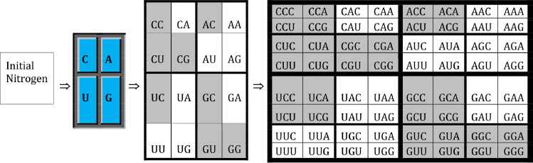
The discovery of the double helix structure of DNA in 1953 [1] led to the rapid development, advances, and growth of genetics in biology. The four letters (or the four nitrogenous bases A, C, G, T/U) of the genetic alphabet form the basis of double helix with pairs of A and T/U, and C and G. The set of these four bases bears the substantial symmetric system of distinctive-uniting attributes (i.e., pairs of an “attribute and anti-attribute”). This system of pairs of opposite attributes divides the genetic four-letter alphabet into three equivalences by all three possible ways:
- 1)
A = C & G = U, this equivalence is based on the attributes: amino-mutating or non-amino-mutating under action of nitrous acid HNO2 [2];
- 2)
C = U & A = G, this equivalence is based on the binary-opposite attributes: one or two “pyrimidine” or “nonpyrimidine” rings;
- 3)
C = G & A = U, this equivalence is based on the attributes: three or two hydrogen bonds materialized in these complementary pairs.
Ian Stewart [3] stated that "life is a partnership between genes and mathematics". This statement offers a general guidance of investigation on relationships between genetic alphabets and mathematical numbers. According to three kinds of biochemical attributes equivalence relation (denoted by symbol “=”), Petoukhov showed that the “elementary” four-letter alphabet of genetic code comprises three binary sub-alphabets [4–6]. The connections between these three genetic equivalences with three fundamental number combinations can be made as follows:
- 1)
1st kind of equivalence: G=U=0, A=C=1, amino-mutating absence/present (0, 1)-combination;
- 2)
2nd kind of equivalence: C=U=1, A=G=2, pyrimidines/purines ring-based (1, 2)-combination;
- 3)
3rd kind of equivalence: A=U=2, C=G=3, hydrogen bonds-based (2, 3)-combination.
Based on these three attributes equivalences and corresponding number assignments, three mapping relations from R = {A, C, G, U} to N = {0, 1, 2, 3} were defined in [7] as follows:
- 1)
α: R →{0, 1} with α (G) = α (U) = 0, α (A) = α (C) = 1;
- 2)
β: R→{1, 2} with β (C) = β (U) = 1, β (A) = β (G) = 2;
- 3)
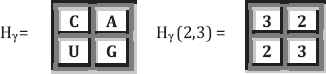
γ: R→{2, 3} with γ (A) = γ (U) = 2, γ (C) = γ (G) = 3.
These three mappings were applied to the standard genetic code in [7] and derived three (8×8) matrices associated with genetic code. The basic symmetrical properties were investigated in [7–10]. In this paper, we investigate the geometric forms and shapes of these three kinds of genetic code equivalences. In Section 2, we show that each equivalence has its own geometric forms and shapes. These forms and shapes include attracting fixed point, repelling fixed point, basin of attractions, Julia sets and corresponding Mandelbrot sets. We further study the golden ratio, ring ratio, and unity ratio matrices associated with genetic code equivalences in Section 3. Conclusion of this paper is summarized in Section 4.
2. GEOMETRIC SHAPES AND FORMS ASSOCIATED WITH THREE KINDS OF GENETIC CODE EQUIVALENCES
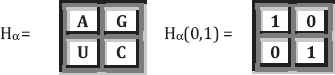
In order to study the geometric forms and shapes of genetic code equivalences, we use three (2×2) square matrices to represent these three kinds of genetic code equivalences:
- 1.
G=U=0, A=C=1, amino-mutating absence/present (0, 1)-combination. Using this numerical mutating value 0 or 1, we arrange this first genetic equivalence as the following 2×2 square matrices:
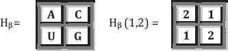
- 2.
C=U=1, A=G=2, pyrimidines/purines ring-based (1, 2)-combination. Using numerical ring values of 1 or 2, we arrange this second genetic equivalence as the following 2×2 square matrices:
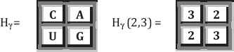
- 3.
A=U=2, C=G=3, hydrogen bonds-based (2, 3)-combination. Using numerical bond values of 2 or 3, we arrange this third genetic equivalence as the following 2×2 square matrices:
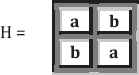
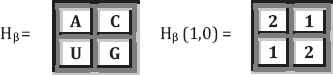
These 2×2 matrices provide building blocks for constructing higher dimensions of matrices of 4×4, 8×8, and so on. In this section, we study these three pairs of basic (2×2) matrices [Hα, Hα (0, 1)], [Hβ, Hβ (1, 2)], [Hγ, Hγ (2, 3)] and establish their mathematical properties.
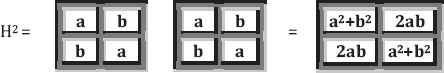
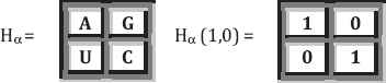
Based on three equivalences of these four alphabets (A, C, G, U), it is easy to see that both diagonal entries of each matrix Hα, Hβ, and Hγ are equal. Thus, we consider the following matrix of H:
Next, taking the square of matrix H gives us:
We now set up the following three equations:
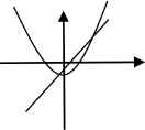
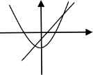
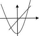
These three systems of equations of a and b are nonlinear. The first equation of each group represents circles with radius R of √1, √2 and √3 respectively (Fig. 1).
Three circles with radius R of √1, √2 and √3 respectively.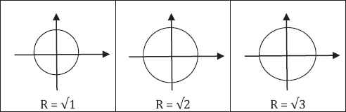
The second equation provides simple relationships between variables a and b:
Solve each pair of equations, we obtain following solutions corresponding to each equivalence equation:
Furthermore, we have the following recursion relations:
The first line of each equation provides a recursive relation of variable a, that leads to the following well-known representation of continued fractions:
The second line of each equation provides another recursive relation of variable a, that leads to the following well-known representation of continued square roots:
Here we note that aα, aβ, and aγ can be also represented in a trigonometric form as follows:
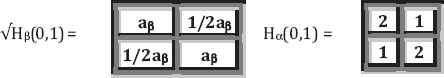
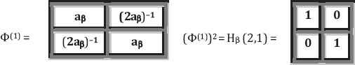
By taking the square root (in common definition) of each H matrix, we obtain the following matrix equations:
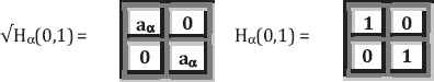
Based on above discussions, we have obtained the following:
Property 1: Three kinds of genetic code equivalences are associated three kinds of mathematical ratios:
- 1.
aα = 1 (here we call it unity ratio) derived from the first kind of genetic attributes: amino-mutating or non-amino-mutating under action of nitrous acid HNO2;
- 2.
aβ = (1 + √3)/2 = 1.36602540378… (here we call it ring ratio) derived from the second genetic attributes of 1 pyrimidines and 2 purines rings;
- 3.
aγ = (1 + √5)/2 = 1.61803398875… (which is the well-known golden ratio ϕ) derived from the third kind of genetic attributes: three or two hydrogen bonds are materialized in these complementary pairs.
The third line of equation is a form of quadratic equation Qc(a) = a2 + c, where c = 0, –½, and −1. Dynamics of this family of quadratic functions Qc(a) = a2 + c have been well studied in the theory of chaos and fractals. These dynamics include attracting/repelling fixed point, attracting/repelling periodic point, basin of attraction, bifurcation, Julia set, Mandelbrot set, orbits, self-similarity, and many more. Here we’ll focus on their basic dynamics.
For each value of c = 0, –½, and −1, we illustrate each quadratic function with some basic dynamics (Table 1).
 |
 |
 |
| c = 0 | c = –½ | c = –1 |
| a2 – 0 = a | a2 – (1/2) = a | a2 – 1 = a |
| Attracting fixed point: 0 | Attracting fixed point: (1 – √3)/2 | Attracting fixed point: (1 – √5)/2 |
| Repelling fixed point: 1 | Repelling fixed point: (1 + √3)/2 | Repelling fixed point: (1 + √5)/2 |
| Basin of attraction: | Basin of attraction: | Basin of attraction: |
| Iα = [–(1 + √1)/2, (1 + √1)/2] | Iβ = [–(1 + √3)/2, (1 + √3)/2] | Iγ = [–(1 + √5)/2, (1 + √5)/2] |
Basic dynamics of Qc (a) = a2 + c for each value of c = 0, –½, and −1.
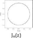
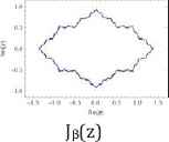
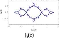
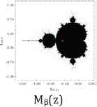
Furthermore, we use common variable z for a and show their Julie sets Qc(z) = z2 + c for each value of c = 0, −½, and −1, associated Mandelbrot sets with specific location of c values (Table 2).
| c = 0 | c = −1/2 | c = −1 |
 |
 |
 |
 |
 |
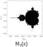 |
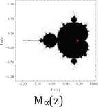
Julie’s sets and Mandelbrot set for each c values of 0, −1/2, and −1.
Based on discussion above, we derived the following:
Property 2: Each c value of 0, −1/2, and −1 from their Julie sets Qc(z) = z2 + c is in the Mandelbrot set. Each attracting fixed points of 0, (1–√3)/2, and (1–√5)/2 is also in the Mandelbrot set. The Julie’s sets for each c values of 0, −1/2, and −1 and for each attracting fixed point are bounded and connected. Furthermore, each Julie set is symmetric with respect to origin and both axes. These three Julie sets satisfy the following relations:
Moreover, the Mandelbrot sets Mα(a), Mβ(a), and Mγ(a) are the same respect to three different positions of c values. As c values decrease from 0 to −1, the corresponding ratios of aα increases from 1 to golden ratio of aγ = (1 + √5)/2 = 1.61803398875… While Mandelbrot sets remain fixed for all c values, the Julie set changes from a unit circle to a symmetrical fractal set.
3. GENETIC MATRICES ASSOCIATED WITH THREE KINDS OF GENETIC CODE EQUIVALENCES
In the previous section, we showed that the third genetic equivalence of hydrogen bonds is connected to the golden ratio ϕ:
In this section, we first pay close attention to the third kind genetic code equivalence with numerical bond values of 2 or 3 as this is connected to a well-known golden ratio. The golden ratio plays an important role in mathematics, science, arts, engineering, and many other fields. It was studied by Leonardo da Vinci, J. Kepler and many other prominent thinkers. A special museum called “Museum of Harmony and Golden Ratio” was established at www.mi.sanu.ac.rs/vismath/stakhov/index.html by A. Stakhov. It documented the golden ratio’s history, development, advances and applications. Recently it was shown in [11] that genetic codon populations in single-stranded whole human genome DNA are fractal and fine-tuned by the golden ratio 1.618. From microlevel of DNA structure to general shape of biological organisms, the golden ratio ϕ = (1 + 50.5)/2 = 1.618… shows up within their compositions and construction. Next, we note that standard genetic code can be constructed by Kronecker product process from a 2×2 to 4×4 and then 8×8 matrices as illustrated [9] in Table 3.
Genetic code matrices.
Golden ratio matrices associated with the third kind of genetic code equivalence: Starting with our 2×2 matrix of golden ratio, we can construct the higher dimensions (4×4 and 8×8) of golden ratio matrices from the following steps.
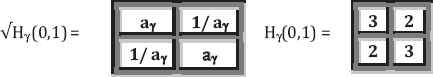
Step 1: The complementary letters C and G have 3 hydrogen bonds (C = G = 3) and the complementary letters A and U have 2 hydrogen bonds (A = U = 2). A hydrogen bonds (2, 3) based equivalence matrices are:
The genomatrices H(2,3)(n) = [3 2; 2 3](n) are based on product of numbers of hydrogen bonds (C=G=3, A=U=2). Here we note that all matrices H(2,3)(n) are nonsingular. They are symmetrical relative to both diagonals and are doubly stochastic. That is the sums of all numbers in the cells of each row and of each column in any matrix H(2,3)(n) are identical to each other.
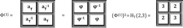
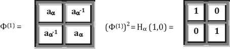
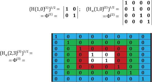
Step 2: Next for each n = 1, 2 and 3, we raise the power ½ in ordinary sense to Φ = (H(2,3)(n))1/2, the matrix elements of which are equal to the golden ratio and to its inverse value (Fig. 2).
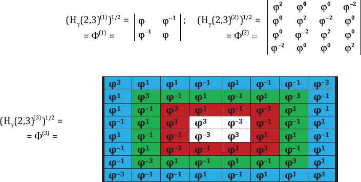 Figure 2
The golden ratio matrices Φ(n) = (H (n))1/2.
Step 3: Taking the square of each golden ratio matrix, we return to the hydrogen bonds (2, 3)-based equivalence matrices.
It is known that proportions of a golden ratio characterize many physiological processes: cardio-vascular processes, respiratory processes, electric activities of brain, locomotion activity, etc. This new theme of the golden ratio in genetic matrices appears to be important because many physiological systems and processes relate to it. It is hoped that these golden ratio matrices could be used for further investigation on the growth and development of genetic code systems.
Using above three steps, we next construct higher dimensions (4×4 and 8×8) matrices of ratios of aα = (1 + √1)/2 and aβ = (1 + √3)/2 associated with the first and second kinds of genetic code equivalences.
Unity ratio matrices associated with the first kind of genetic code equivalence: The resulting matrices have the same structure and symmetrical properties as the golden ratio matrices (Fig. 3).
The unity ratio matrices Φ(n) = (H (n))1/2.
The beginning of the Kronecker family of the unity matrices Φ(n) = (Hα(n))1/2, where aα = (1 + √1)/2 = 1 is the unity ratio.
Ring ratio matrices associated with the second kind of genetic code equivalence: The resulting ring ratio matrices have the same structure and symmetrical properties as the golden ratio matrices (Fig. 4).
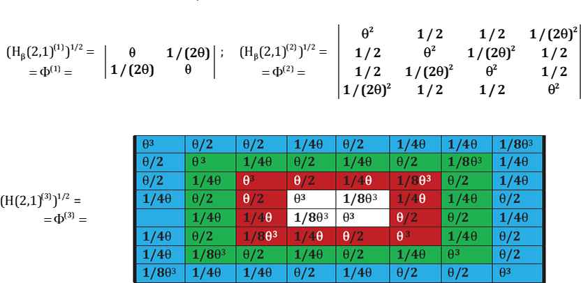
The ring ratio matrices Φ(n) = (H(n))1/2.
For a notation simplicity, we denote θ as aβ, called as a ring ratio θ = (1 + √3)/2.
The beginning of the Kronecker family of the ring matrices Φ(n) = (H(n))1/2, where θ = (1 + √3)/2 = 1.366…. as a ring ratio.
Further examining row and column entries of these three kinds of unity ratio, ring ratio, and golden ratio matrices, it is easy to see that these three matrices have the following property.
Property 3: These three kinds of matrices associated with three kinds of genetic code equivalences are doubly stochastic and have the common sums (rows and columns) as summarized in Table 4, Table 5 and Table 6.
| (1,0)-Matrices With Unity Ratio of a α = 1 | Common Sums | Sqrt of Matrices | Common Sums |
|---|---|---|---|
| Hα (1,0) (1) | 1 | (Hα (1,0) (1)) (1/2) | 1 |
| Hα (1,0) (2) | 1 | (Hα (1,0) (2)) (1/2) | 1 |
| Hα (1,0) (3) | 1 | (Hα (1,0) (3)) (1/2) | 1 |
(1,0)-Matrices with unity ratio of aα = 1.
| (2,1)-Matrices With Ring Ratio aβ = (1 + √3)/2 | Common Sums | Sqrt of Matrices | Common Sums |
|---|---|---|---|
| Hβ (2,1) (1) | 3 = 3 1 | (Hβ (2,1) (1)) (1/2) | (√3) 1 = 3 1/2 |
| Hβ (2,1) (2) | 9 = 3 2 | (Hβ (2,1) (2)) (1/2) | (√3) 2 = 3 |
| Hβ (2,1) (3) | 27 = 3 3 | (Hβ (2,1) (3)) (1/2) | (√3) 3 = 3 3/2 |
(2,1)-Matrices with ring ratio aβ = (1 + √3)/2.
| (3,2)-Matrices With Golden Ratio aγ = (1 + √5)/2 | Common Sums | Sqrt of Matrices | Common Sums |
|---|---|---|---|
| Hγ(3,2) (1) | 5 = 5 1 | (Hγ (3,2) (1)) (1/2) | (√5) 1 = 5 1/2 |
| Hγ (3,2) (2) | 25 = 5 2 | (Hγ (3,2) (2)) (1/2) | (√5) 2 = 5 |
| Hγ (3,2) (3) | 125 = 5 3 | (Hγ (3,2) (3)) (1/2) | (√5) 3 = 5 3/2 |
(3,2)-Matrices with golden ratio aγ = (1 + √5)/2.
4. CONCLUSION
In summary, we have demonstrated the geometric shapes and forms of three kinds of genetic code equivalences with three kinds of golden ratio matrices, unity ratio matrices, and ring ratio matrices as stated in Property 1 and Property 2. Furthermore, these three kinds of genetic matrices are doubly stochastic as noted in Property 3. These connections illustrate the biological organisms’ self-production and self-similarities phenomena. These connections may lead to new understanding of genetic code systems. Many literatures on the connections between mathematics numbers/ geometries and biological systems have emerged in recent years [12,13] to further advance our understanding of life and its evolutions [14,15].
Conflict of Interest
The author declares no conflicts of interest.
Author Contribution
This article and the underlying research were independently completed by Matthew He.
Funding
The author declares that no funding was used for this study.
Data Availability
Not applicable to this article as no additional underlying data were created or analyzed in this study.
REFERENCES
Cite This Article
TY  - JOUR
AU  - Matthew He
PY  - 2023
DA  - 2023/07/12
TI  - Geometric Shapes and Forms Associated With Three Kinds of Genetic Code Equivalences
JO  - Growth and Form
SP  - 11
EP  - 20
VL  - 4
IS  - 1-2
SN  - 2589-8426
UR  - https://doi.org/10.55060/j.gandf.230712.001
DO  - https://doi.org/10.55060/j.gandf.230712.001
ID  - He2023
ER  -


