
Revised 10 July 2023
Accepted 23 October 2023
Available Online 29 November 2023
- DOI
- https://doi.org/10.55060/s.atmps.231115.013
- Keywords
- Complexity
Superellipses
Superformula
Gielis Transformations
Natural shapes and phenomena - Abstract
Our scientific and technological worldviews are largely dominated by the concepts of entropy and complexity. Originating in 19th-century thermodynamics, the concept of entropy merged with information in the last century, leading to definitions of entropy and complexity by Kolmogorov, Shannon and others. In its simplest form, this worldview is an application of the normal rules of arithmetic. In this worldview, when tossing a coin, a million heads or tails in a row is theoretically possible, but impossible in practice and in real life. On this basis, the impossible (in the binary case, the outermost entries of Pascal's triangle
- Copyright
- © 2023 The Authors. Published by Athena International Publishing B.V.
- Open Access
- This is an open access article distributed under the CC BY-NC 4.0 license (https://creativecommons.org/licenses/by-nc/4.0/).
1. RETHINKING ENTROPY AND COMPLEXITY IN NATURAL SYSTEMS
1.1. Kolmogorov and Shannon
Entropy is originally a concept from thermodynamics that distinguishes between useful and useless energy1. This led to the Second Law of Thermodynamics, which states that entropy always increases. The Hamiltonian principle states that the differential equation for the Second Law is equivalent to the integral equation for Least Action.
In the information age, entropy has been found to be related to complexity. There are two main approaches, one of which is based on C. Shannon (1916–2001) and the other on A.N. Kolmogorov (1903–1987). The former is communication theory, while the latter is the basis of Algorithmic Information Theory (AIT), which studies the shortest algorithm for encoding a message that yields the “best possible compression”.
This is of course also usage-based and refers to 'optimal' methods of data processing. The commonly used example is a particular sequence of binary digits, symbols or characters. Each of these sequences is called a message. Two sequences (or strings) are:
Kolmogorov focuses on the shortest path to encode the message (to define complexity), while Shannon estimates the odds of what the next letter (A or B) in the transmitted message will be. Shannon's communication theory focuses on a sender of a message, the communication or transmission channel, and a receiver of the message. For message 1, the sender can simply encode the message as “AB & repeat 11 times”; this message is not complex, neither for the sender nor for the receiver. For the second series, the situation is quite different. If the sender has sent the first ten symbols of the series, the receiver of the message has no way of knowing whether the next (11th) letter to arrive over the transmission channel will be A or B. This is a surprise. Each next letter is a surprise with a 50/50 chance of being A or B, with equal probability for A and B.
From Kolmogorov's point of view, the first message is simple: it has low complexity, both from the sender's and the receiver's point of view, based on the rules of arithmetic (with multiplication: 11 times AB). Because of the repetition, this message has high redundancy, the opposite of complexity. The second message, on the other hand, has high complexity because it cannot be encoded in a simpler way than transmitting the entire message letter by letter. From Shannon's point of view, the second message is the least predictable. In these theories, statements about predictability, complexity and entropy are equivalent [1,2]. Message 2 has the “least predictability” and is the “most complex message”; it also has the highest entropy. Message 1 is simple and has low complexity. One could also say that message 1 has a clear structure, while message 2 lacks structure. A more formal comparison:
“Kolmogorov complexity K(x) and Shannon Entropy H(x) are conceptually different, as the former is based on the length of programs and the latter on probability distributions.
The Kolmogorov complexity K(x) measures the amount of information contained in an individual object (usually a string) x, by the size of the smallest program that generates it. It naturally characterizes a probability distribution over Σ (the set of all finite binary strings), assigning a probability of
The Shannon entropy H(X) of a random variable X is a measure of its average uncertainty. It is the smallest number of bits required, on average, to describe x, the output of the random variable X.
However, for any recursive probability distribution (i.e. distributions that are computable by a Turing machine) the expected value of the Kolmogorov complexity equals the Shannon entropy, up to a constant term depending only on the distribution.” [1]
1.2. Archimedes, Pascal, Leibniz and Mendel
Using the symbols or letters A and B is similar to flipping a coin. In a Bernoulli procedure, where a fair coin is tossed, the 'probability' of heads or tails can be read from Pascal's triangle, which encodes the arithmetic rules
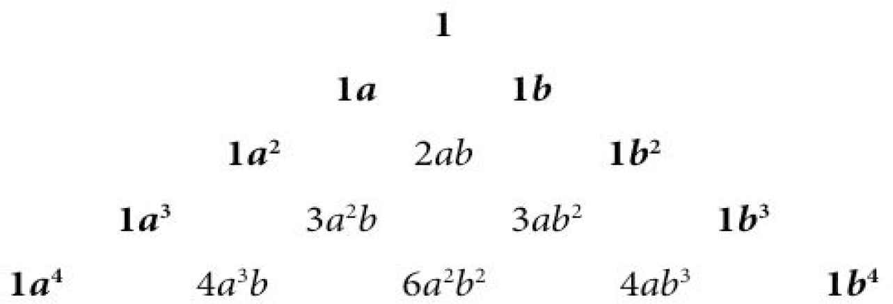
Pascal’s triangle.
If you flip a coin 100 times, you can calculate which outcome has the highest probability. H(eads) is then a and T(ails) is b. The law of large numbers (if you repeat the same experiment multiple times) ensures that a series of 50 times heads and 50 times tails (without specifying the exact sequences) will occur most often if you repeat the experiment. In any case, this will occur much more often than 100 times heads or 100 times tails as a result. The probability of this would be extremely low. Using Pascal's triangle, it is also easy to determine the probability that a row contains 38 times heads and 62 times tails (or vice versa). In Fig. 1, the first five rows are shown to illustrate the simpler cases. If you flip the coin 2 times, you have 2 chances out of a total of 4 that you will get HT or TH. The number 4 is the sum of all coefficients in row 3. The chance of hitting HH is 1 in 4, and the same is true for TT.
If you flip the coin 4 times, there are 16 possible outcomes, with 6 chances out of a total of 16, for a result with 2 heads and 2 tails. The exact order of Hs and Ts is not fixed, and they can occur in combinations such as HHTT or HTHT, with 2 of each. However, the probability of getting HHHH is only 1 in 16, or
Note that a and b can be anything in Pascal's triangle. It can be a = A, b = B; for flipping a coin: a = Heads, b = Tails; or a = 1, b = 0. The latter encodes the binary system going back to G.W. Leibniz (1646–1716), which consists of numbers like 1001111. If you combine 1 and 0 in four different ways (line 5 in Fig. 1) you get 0000 or 1111, or 1001, 1100, 1010, 0101, 0110, 0011 or... The latter are 6 possible combinations of 2 times 1 and 2 times 0, while the former are pure sequences of 0 and 1. This binary or Boolean logic [3] is the basis of our modern computers, where electronic gates are switched on or off.
Mendel's laws of genetics follow the same arithmetic. With dominant A and recessive a alleles, a monohybrid cross (only one trait) produces three different genotypes: a homozygous dominant AA, two times heterozygous Aa and a homozygous recessive aa. A dihybrid cross (with two traits) with genotypes AA, Aa/aA and aa generates 16 possibilities, corresponding to the fifth line of Pascal's triangle. This emerges from the Punnet scheme, a simple square table or matrix for combining A and a. Because of the dominance of the genes, the genotype will express the trait if only one of the alleles is dominant. Thus, in a dihybrid cross, you get a ratio of 9:3:3:1. There is only one sibling that has all recessive alleles for the two traits, six siblings that have a trait with two recessive alleles, and nine siblings that have at least one dominant allele for each trait. The work of G. Mendel (1822–1884) is one of the most important milestones and quantum leaps in the history of science. It works because it is arithmetic.
From an arithmetic viewpoint
This means that for any integer value of
The ‘arithmetic’ shift from multiplication of variables to independent events led to a probabilistic worldview [4,5].
1.3. Simon Stevin’s Geometrical Numbers
Beyond arithmetic, the geometrical meaning gives more freedom. One could say that a cube with sides
Higher order expansions can be viewed in the same perspective (Fig. 2). Using
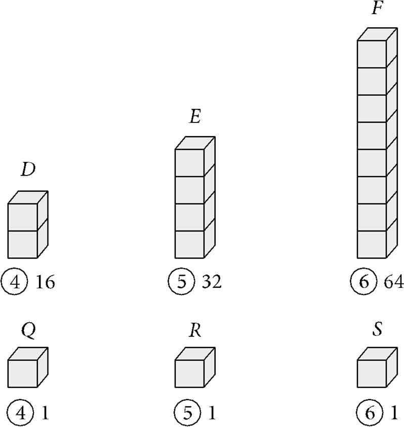
Simon Stevin’s geometrical numbers [6].
About Blaise Pascal, the French mathematician and philosopher, H. Bosmans wrote: “To speak about four-dimensional space is a language that should not offend intelligent people, since it is really only a multiplication. In other words, we would say today that this is only a conventional language referring to a very clear arithmetic operation.” [7] The rules of arithmetic that encode the rules of multiplication (and their interpretation as geometric numbers) also lead to the rules of differentiation and to special functions, regardless of order or dimensions [4,8].
1.4. Apollonius, Descartes, Gauss and Riemann
Using the rules of arithmetic and interpreting subsequent actions in this way is the foundation of a wide variety of scientific methods using probability and combinatorics. An important development with the same rules led to another foundation of the sciences, with focus on “quadratic equations”, i.e. up to the third row
This started with René Descartes (1596–1650), in which the coefficients in the expansion are generalized. Indeed, Descartes’ definition of conic sections, advancing beyond the great geometer Apollonius, can also be considered as a sum of the first three rows of the triangle of Pascal, but now with general coefficients
When this sum equals zero, we obtain the general form for conic sections and the value of the discriminant
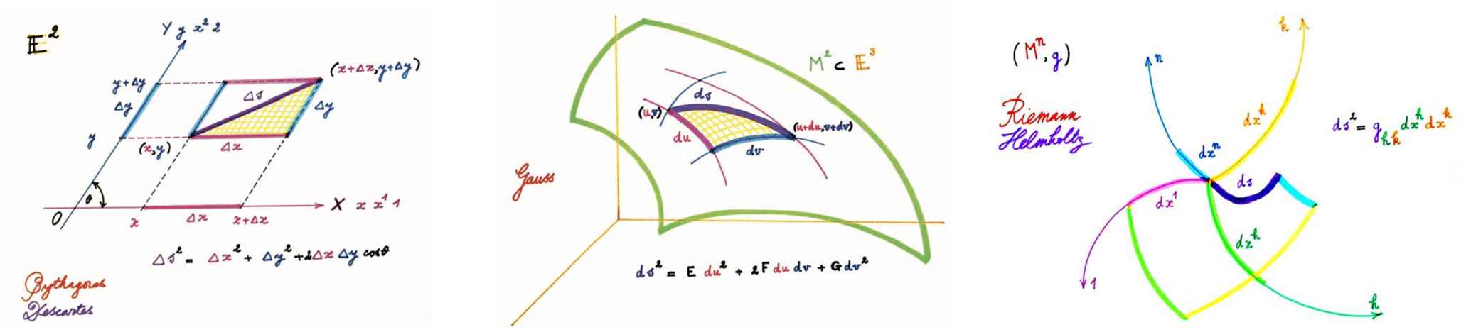
From the Pythagorean theorem to measurements on manifolds [9].
The determination of coefficients
Interestingly, B. Riemann not only showed how rigid bodies behave in a predefined space, but also how space is affected by rigid bodies, and thus space is an entity subject to the same scientific investigations as bodies [10]. Almost 60 years later, A. Einstein (1879–1955) showed that “matter tells space how to curve, and that space tells matter how to move”.
And it is the definitive beginning of submanifold theory as we know it today, of surfaces and bodies of a certain dimension living in higher dimensional surfaces and bodies. But most importantly, it is our experience that makes it the space of our geometry and physics, with the projective and metric relationships. We leave this brilliant generalization of the Pythagorean theorem and return to the combinatorial strategy.
2. STRUCTURE AND VARIATION
2.1. Turing Machines, Normal Distributions and Thermodynamic Entropy
Since the same binomial theorem underlies the binary number system (for
The key of Turing machines is that a message can be transmitted which, in the case of message 2, runs through the entire series step by step, stopping after the last letter. Thus, until the complete message is received, there is no way to know exactly what the message is. Message 2 has high complexity, or associated with it according to information theory, high entropy. The same machine can easily encode message 1 as 11 times AB. This is no surprise and therefore the series of message 1 has low complexity and associated low entropy.
The process of tossing a coin is the simplest example of a Bernoulli process dealing with discrete processes. For very large numbers, the process can be approximated by the normal distribution curve. The law of large numbers states that for 500 billion coin tosses, the most likely outcome is 250 billion times heads and as many times tails. On the other hand, it is extremely unlikely that 500 billion times heads H or 500 billion times tails T will fall. Also 490,000,000,000 heads and 10,000,000,000 tails can be neglected, etc. The sequences HHH....HH and TTT....TT are at the extreme left and right ends of the distribution and have a very, very low probability of occurring. This possibility can simply be ignored.
More generally, a Bernoulli process is modeled by a random variable that can take only two values, and not simultaneously (Fig. 4). From the Bernoulli process with probability p for one of two values, one can define a binary entropy function
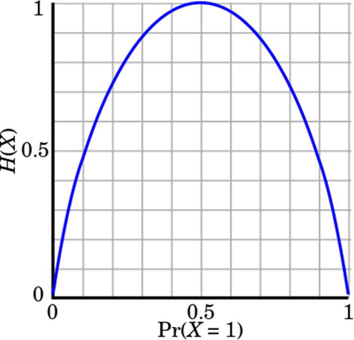
Entropy function for a Bernoulli process.
The outcomes HHHHHHHH… or TTTTTTTT… have zero entropy (equivalent to ‘lowest complexity’ or ‘highest structure’). In fact, if we look at the left and right entries of Pascal’s Triangle in subsequent rows (
2.2. Ensembles and Individuals
The Second Law of Thermodynamics states that entropy keeps increasing. In other words, the states with the highest entropy are always the most probable. The universe is heading for a heat death without any structure. Structures or pockets in space with low entropy are possible, but the general trend is toward complete structurelessness. If we take a step back, we see that the whole probabilistic approach to physics introduced by Boltzmann underlies the scientific method of our time, and statistical thermodynamics, which led to the Second Law, is a perfect example.
Entropy is often associated with disorder, but it is more correct to say that all correlations between objects (including causal correlations) are removed from consideration with the foundations established by Kolmogorov. We can view gas simply as a collection of spheres constantly bumping into each other (and more so the higher the temperature), but that is all they do; no interactions. It is the behavior of these spheres that leads to macroscopically measurable quantities such as temperature or pressure. The key ingredient of statistical thermodynamics is the “indistuingishability” of the objects, and this is the same in quantum mechanics [11].
In this sense, Erwin Schrödinger (1887–1961) once said that all laws of physics are statistical laws [12]. According to Schrödinger, the ’individual’ plays no role in science [13]. However, it is the ‘individual’ that interests us, and the individual may be the most unlikely among the possibilities within the statistical laws of nature. Indeed, in recent years multiple lines of evidence have emerged showing what is most unlikely, or most rare or extreme, is widely encountered in nature, in all of its forms and phenomena.
Our probabilistic worldview is indeed only one way of looking at the world. Another way of studying nature is possible. Using a new and completely different set of glasses and lens, originally developed by Gabriel Lamé, provides a much clearer view. In nature one finds many instances of fully biased processes. I will refer to this as Lamé’s footprint in nature, for reasons to be detailed further. Surprisingly, both the probabilistic view and the new view use the same computational rules but apply them differently.
2.3. Entropy in Double-Stranded DNA
Let us start with a counterintuitive example, namely the entropy of double-stranded DNA. A single strand of DNA is a series of four bases of purine (adenine A and guanine G) or pyrimidine (thymine T and cytosine C) type, for example, …AGTCGGTTAACGACT…. The sequence of the four bases in DNA is not random. Specific sequences of three DNA-bases, known as triplets, are the blueprints for building proteins. It is the genetic code of life itself.
From Mendel’s Laws to the genetic code is actually only a small step. Extending this to the representations of four nitrogenous bases and triplets in the form of eigenvalues returns the alphabet of 64 triplets, and the partition into sub-alphabets of 32 triplets leads automatically to the genetic code with many mathematical regularities [14,15]. When expressed as tensor products of matrices and eigenvalues [16], this shows that the genetic code itself is based on the same rules of arithmetic encoded in Pascal’s Triangle.
DNA carries the necessary genetic information to build living organisms, and in this sense, one can estimate the information content of DNA. Since sequences of the four bases are certainly not random and DNA strands have a lot of redundancy, it is not straightforward to determine or calculate entropy in DNA [17,18,19]. However, it can be stated with confidence that the information content (and its entropy) is high. It is certainly not zero, as one could expect from long streaks of ...AAAAAA... or ...GGGGGG.... Now, a sequence in one strand of the DNA molecule is very similar to a binary digit series, consisting of 0s and 1s. One can assign 0 to the pyrimidine bases and 1 to the purine ones. Consider then a series of 1s and 0s, such as 101 000 101 010 000 100 111 00, with very low to no predictability (in any case it was typed as a random series): its entropy or information content is very high.
However, DNA itself is a double-stranded molecule and the four bases always occur pairwise. A purine always pairs with a pyrimidine base and they do so exclusively. A(denine) always pairs with T(hymine) and C(ytosine) always with G(uanine). These complementary strands form the backbone of double-stranded DNA. The base pairs occupy approximately the same space, which enables a twisted DNA double helix formation without distortions. Pairing between A and T is via two hydrogen bonds, whereas G and C are paired via three hydrogen bonds and these hydrogen bonds stabilize the double helix.
The surprising fact now is that the entropy of the DNA molecule itself is zero, precisely because of its double stranded nature, with each strand complementary to the other strand. Indeed, when we pair to the original strand the complementary one in 1 and 0, we obtain a structure depicted below.
Applying the rules of binary operations pairwise in the two strands (1 or 0 in the upper strand, to its counterpart in the complementary lower strand), with 1 + 0 = 1 and 0 + 1 = 1, we find that the double-stranded series is 111 111 111 111 111 111 111 111. This series is no other than always 1, very simple, no surprises, as if obtained with a fully biased coin. This corresponds to the highest possible structure or zero entropy for the DNA molecule!
The high information content in single DNA strands is actually safeguarded by having the same information in the complementary strand. At least two other aspects add to this remarkable stability of the DNA molecule. First, it aligns with the helical structure of double-stranded DNA wherein the molecules try to minimize overall and local stress [20]. Second, in eukaryotes, DNA is wrapped tightly around histones, forming chromatin and is safely guarded in the nucleus of cells, providing for additional layers of protection of the information content in DNA. Hence the high information content in single DNA strands (with high entropy) is safeguarded by building a structure with no information at all (and zero entropy): the DNA molecule. While our probabilistic worldview focuses on maximal entropy, it turns out that nature also prefers biased coins.
One further example of “adding the exceptional” and “biased coins” is found in hybrid breeding in plants. By crossing two inbred parents, hybrids have a combination of traits from both parents that allows the hybrids to have an overall performance that exceeds the performance of either inbred parent.
The “exceptional”, i.e. the left and right ends of the triangle, is homozygosity in the case of genetics and it is obtained by exclusive self-pollination over multiple generations. This inbreeding results in diploid organisms, with both alleles of a gene either both dominant A or recessive a, so you have aa or AA. Targeted breeding efforts by inbreeding, aim at lines that are homozygous (recessive or dominant) in a number of genes, namely
The double-stranded nature of DNA exemplifies the tendency of nature to search for ultimate structure and stability. Information and structure go together. In the case of DNA, structure safeguards information. In hybrid breeding the low information content (low genetic diversity) in inbred lines is exploited in crosses to create very great diversity (high information). In natural processes, the reduction of complexity by having more structure goes together with increased information content within this structure.
3. THE FOOTPRINT OF GABRIEL LAMÉ
3.1. Supercircles and Superellipses
Returning to Pascal’s Triangle, instead of focusing on the most likely we can combine the least likely from both ends, namely
In supercircles (Fig. 5) or superellipses for
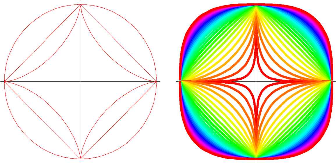
Supercircles as examples of Lamé curves for various n.
This works also for “larger circles” when
This can also be extended in higher dimensions. For example,
The original Pythagorean Theorem defines all possible circles for any radius based on the right triangle. This brilliant move by Pythagoras reduced all circles (and also all conic sections by projective equivalence) to this one notion of the Euclidean circle. This is the basis of (almost) all our scientific methods (direct or hidden) with a strong reduction of complexity. By introducing redundancy, it allowed us to gain information. Furthermore, Gabriel Lamé's brilliant move of generalizing only the exponent of the circle greatly reduces complexity. A single additional parameter besides the magnitude, expressed by R or A and B, is sufficient. Many examples will be given later in this article proving that supercircles are an excellent model for forms and phenomena of nature. This model was tested on more than 40,000 specimens [26].
3.2. Lamé Curves, Modular Arithmetic and Power Laws
In fact,
How can one reconcile the extreme unlikelihood of
The best strategy is to focus on the same foundations, the same rules of arithmetic.4
We can take the complementary view (or the completely opposite view depending on the choice of words) to the 'scientific' view, which is based on the same binomial expansion. Indeed, if we slightly rearrange the results of the arithmetic rules in each line of Pascal's triangle as in Eq. (3), we find that we can neglect the part between the square brackets (the non-Lamé part). We do not need these products of x and y raised to a power at all, only the Lamé-part
Using the above example, we only use the classical “modular arithmetic”5 part:
So, for the binomial expansion
Note that in Lamé curves
| Variables | Planar Curves | Types | Special Means |
|---|---|---|---|
| Supercircles & Superellipses | Lamé curves | Arithmetic mean
|
|
| Superparabolas & Superhyperbolas | Power laws | Square of geometric mean
|
Lamé curves and power laws as generalizations of conic sections [27].
3.3. Allometry, Laws of Physics and Production Functions
In the same way as supercircles are generalizations of circles, these power relations are superparabolas, generalizations of the classic parabola
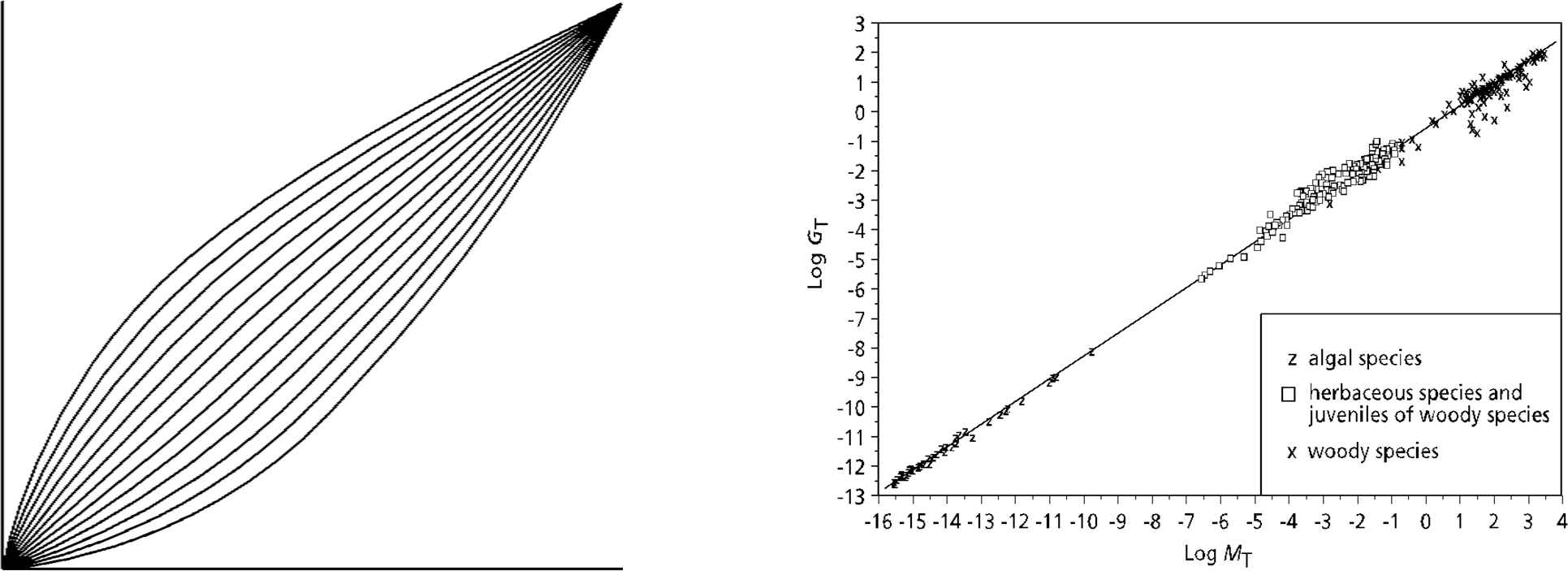
All power laws have these simple graphical expressions, but they are usually disguised as straight lines using logarithmic transformations. Fig. 6 right shows the allometric relationships between biomass and metabolism in plants over a wide range of plant sizes, from small algae to the largest trees [28]. Fig. 7 shows such relationships in planets, codified in Kepler's laws.
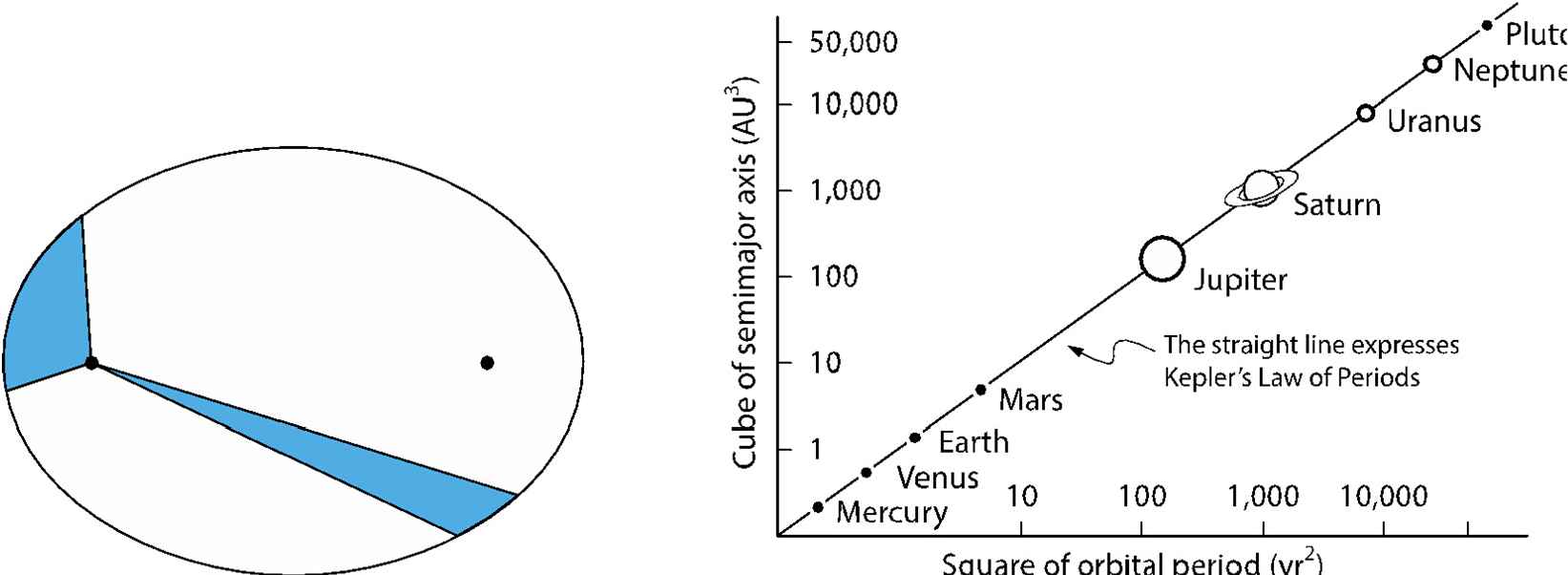
Kepler’s law of equal areas in equal times (left) and his law on the square of the orbital period vs. the cube of the semi-major axes of the elliptic orbit (right) [5].
Allometric laws are called laws because they do the same thing as the laws of physics, which is to reduce complex relationships to simple relationships between two measurable quantities. These relationships can be linear, or the quantities can be raised to a power (e.g. in Kepler's Law of Equal Areas, Fig. 7). Such allometric laws can be found everywhere [29]. In the last 20 years, an enormous number of empirical allometric relations have been revealed at all levels, from the giant to the small and for living and non-living entities, and the underlying geometry turns out to be very simple [27,30]6.
Also in economics such power laws are everywhere, from the size of cities to the power noise in time series. A prime example of allometry in economy is the Cobb-Douglas production function, with the output of a process defined by Capital and Labor
One other metric in economy is the Gini index to quantify inequalities based on Lorenz curves. In many cases this can be modeled efficiently with Lamé curves or superellipses [34,35]. Recently, it was shown that Gini and Theil indices from economy can also be used in the study of natural phenomena. While leaves themselves can be modeled with superellipses, their distribution on whole plants can be modeled with Gini indices [36,37]. Lamé curves are found everywhere [38].
3.4. Lamé’s Footprint in Ecology and Geometry
In 1993, another example of the Lamé footprint was introduced in biology and ecology: the so-called Antonelli metric [39]. This has its origin in Finsler geometry, a geometry that is not limited to the generalization of the Pythagorean theorem as in Fig. 3. It can even be considered as “Riemannian geometry without the quadratic constraint” [40].
Peter L. Antonelli (1941–2020) wrote [41]: “As is well known, Riemann foresaw the advent of Finsler geometry (the 1918 thesis of P. Finsler, a student of Carathéodory) when he gave in the cited reference an example of a line-element defined as the 4th root of the sum of 4th powers of the independent coordinate increments, which contrasted sharply with the familiar Pythagorean expression
This ecological metric was first mentioned in [42] and it is worth noting that this is also directly related to allometric laws because of the exponential function in the metric. Inspired by Lamé curves, the same metric has been used in the study of seismic wave propagation [43], whereby the indicatrix expresses the anisotropy of the shape of the seismic wavefront.
This also provides an opportunity to place this whole development into the historical framework of the first half of the 19th century and the role of G. Lamé. He was one of the first to introduce curvilinear coordinates for surfaces. The importance of the curvilinear coordinates introduced by Riemann for mathematics and physics is explained by E. Cartan (1869–1951) [44]: “Euclidean geometry also knows analytical methods based on the use of coordinates, but these coordinates (Cartesian, rectangular, polar, etc.) have a precise geometrical meaning, and this is why their introduction can only take place once geometry is founded by its own methods. In Riemannian geometry, on the other hand, the coordinates, introduced from the beginning, are simply used to locate from an empirical way the various points in space, and the purpose of geometry is precisely to identify the geometrical properties that are independent of this arbitrary choice of coordinates. A problem of this nature is not absolutely new. Gauss, in his “Disquisitiones generales circa superficies curvas”, had precisely given a model for the development of two-dimensional Riemannian geometry”.
Cartan continues: “On the other hand Lamé, a few years after Riemann’s Dissertation, it is true, had, for three-dimensional Euclidean geometry, introduced coordinates that were not as general as those of Riemann, but within this somewhat more restricted framework, he was, in short, doing Riemannian geometry. The need to use arbitrary coordinate systems had a profound influence on the further development of Mathematics and Physics. It led to the admirable creation of the absolute differential calculus of Ricci and Levi-Civita; this calculus itself was the instrument that served for the elaboration of general relativity”.
Thus, according to Élie Cartan, Gabriel Lamé should be considered as one of the co-founders of Riemannian geometry. René Guitart comments on the note of Cartan [45]: “Since Riemann’s Dissertations are from 1851 and 1854, it is understandable that Cartan is thinking here of Lamé’s treatises, which are later, notably the treatise on curvilinear coordinates of 1859. But in fact Lamé’s ideas about curvilinear coordinates are already in place in his articles of the 1830s, and thus precede Riemann’s work, which gives even more importance to Cartan’s appreciation. However, as Darboux points out, symmetrical and isothermal curvilinear coordinates on surfaces were introduced by Gauss in 1825, in relation to the question of the representation of a surface on a plane while preserving angles (question of geographical representations). … Finally, by “arbitrarily” parameterizing space, as Euler parametrized curves and Gauss the surfaces, Lamé’s curvilinear coordinates were to be the indispensable tool of differential geometry, Riemannian or not, and in particular to allow the development of the method of the répères mobiles”.
It has already been mentioned that Riemann invented the Riemann-Finsler metric, but it is clear that the Lamé curves date from 1818, with the m-th root of a sum of m-th powers (Table 1). Lamé curves and the associated methods for measuring distances are widely used today in mathematics, science and engineering, but are not always recognized as such because they appear under different names. For example, in
Distances thus defined are also called Minkowski distances. For
This all relates to classical means (arithmetic, geometric), conservation laws (e.g. Pythagorean Theorem), conic sections and distance-based geometries (Euclidean, Minkowski) with distance functions of the type
Power laws are used to understand diversity in nature (both animate and inanimate), but studies have shown that Lamé curves are also ubiquitous in nature and far more common in biology than circles or ellipses, which form the basis of the mathematization of nature. The footprint of Lamé has become obvious and adding power laws to this drastically reduces complexity, with conic sections at the core once more. Moreover, it is now clear that we can use it to reduce complexity and gain information, both in geometry and in the natural sciences. A few numbers suffice for the description of shapes and size information.
4. GIELIS CURVES AND TRANSFORMATIONS
4.1. A Generic Geometric Transformation That Unifies a Wide Range of Natural and Abstract Shapes
The model used to approximate bamboo culms [47] and tree rings [48] is actually a modified version of the Lamé curves or a version of the so-called superformula (SF), also known as Gielis Transformations (GT) [5,24]. They are a generalization of Lamé curves, and hence of the circle and the Pythagorean theorem. These are defined by:
For
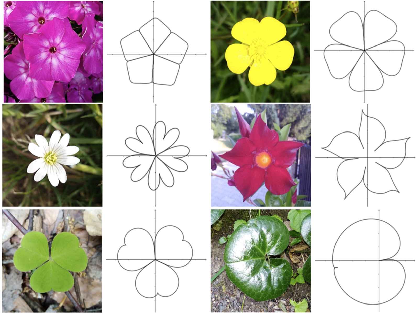
Different leaves and flowers with the Superformula [54].
However, even in the low-parameter version of Eq. (5), with
This SGE has been applied in a variety of studies in bamboo and plants. Interestingly, the fact that only two numbers are needed to describe such curves, one for size and one for shape, means that for a variety of leaves measuring the length and width of the leaves is sufficient to determine the area with sufficient accuracy using Montgomery’s equation, the scaled product of length and width. The so-called Montgomery’s law has now been shown to be valid for a wide variety of plant leaves.
Such simple but accurate measurements have led to a better understanding of leaves and their role. Moreover, widely used descriptive terms such as elliptic, linear or lanceolate to describe leaf shape can now be accurately quantified using only two numbers. It has been successfully tested and validated on more than 40,000 specimens. Gielis Transformations have thus evolved from a stage of “analogy” to a sound scientific method for detecting and validating the footprint of Lamé in nature.
4.2. Square Bamboos Revisited
More than 180 years separate Gabriel Lamé’s original idea of applying Eq. (2a) and Eq. (2b) to crystals from the discovery of a wide range of natural forms described by superellipses. In 1993, superellipses were associated with square bamboos, specifically with the cross-sectional forms of the square bamboo, Chimonobambusa quadrangularis. This was based on an analogy: the shapes of the plants looked very similar to superellipses, a simple model, but now this has evolved into a full scientific methodology for modeling tree rings, leaves and seeds. Two centuries after the original publication by Gabriel Lamé in 1818, the model has also been tested on 30 adult culms of Chimonobambusa utilis, another square bamboo [47]. For 750 sections, both the outer and inner shapes can be modeled with arbitrary accuracy using only a few numbers. A single equation with two parameters and an additional transformation parameter fits all 1,436 inner and outer rings tested (Fig. 9).
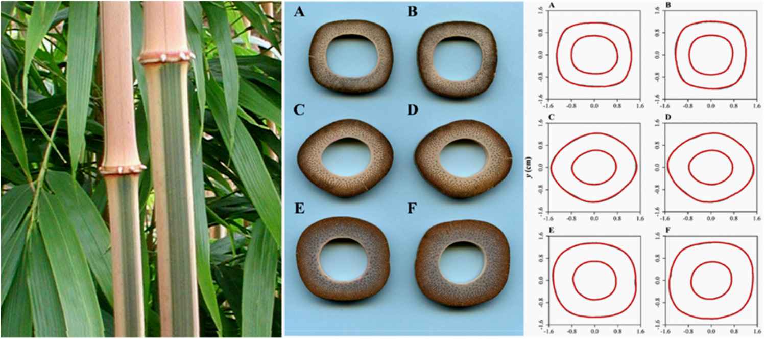
Left: culms of a variegated form of Chimonobambusa quadrangularis. Center and right: fitted curves for the six actual cross-sectional examples of Chimonobambusa utilis (center) using the superellipse equation with a deformation parameter. The grey curves are the actual outer and inner rings; the red curves are fitted curves [47].
When square bamboos, which have been known in China and Japan for thousands of years, came to the attention of Western botanists, it caused a sensation. In 1885 Thiselton Dyer wrote in Nature [55]: “The cylindrical form of the stems of grasses is so general a feature in the family that the reports of the existence in China and Japan of a bamboo with apparently four-angled stems have generally been regarded as myth, or at least as due to some disease or abnormal condition of a species whose stems, when properly developed, have a round cross-section. Of the existence of such a bamboo there cannot, however, now be any kind of doubt”.
Two centuries after Lamé, superellipses are found everywhere. One can rephrase Dyer’s statement as follows: “Of the existence of such superellipses in nature, there cannot, however, now be any kind of doubt”.
5. THE COMPLEX AND THE UNIQUE
5.1. Shape Complexity Revisited
Eq. (4) can be extended to any dimension in various ways, for example, in parametric coordinates:
Depending on the size of the two cross-sections defined by Eq. (4), i.e.
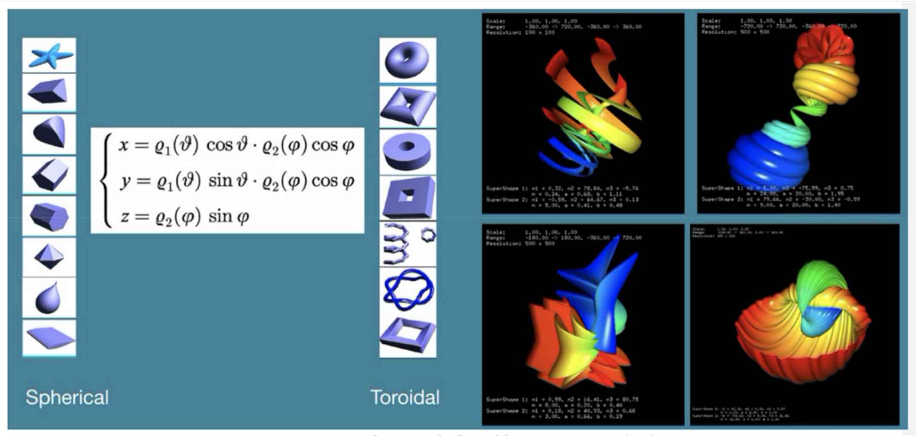
3D shapes.
5.2. Saint-Gabriel
Lamé curves form a bridge between classical Euclidean geometry and Riemannian geometry (with a “quadratic” form based on Pythagoras) on the one hand, and Finsler geometry (“without the quadratic restriction”
) and metric spaces (“with the
In the second half of the 19th century and in the beginning of the 20th century, many great mathematicians were well acquainted with Lamé curves. These curves have a clear relation to the Last Theorem of Fermat. Felix Klein wrote: “The assertion of Fermat means, now, that these curves thread through a dense set of the rational numbers, without passing through a single one except on the axes” [56].
Gauss also knew Lamé’s work well and in fact considered Lamé as the best French mathematician of his time [57]. Knowing that Gauss rarely praised others and the fact that France had a number of first-class mathematicians, this is remarkable. It is a strange twist of history that Eq. (4) took so long to discover [5]. Indeed, Lamé’s supercircles in polar coordinates and Gauss’ Arithmetic-Geometric Mean (Eq. (7)) and his form for computing elliptic functions of the second kind (Eq. (8)) are very closely related (compare with Eq. (4) for exponents equal to 2 and
Gabriel Lamé (Fig. 11) is a central figure in the history of modern mathematics [39] and his work is the inspiration for all of the above, especially the dual view of patterns and of individuals. He spent the third decade of the 19th century in Saint Petersburg, at a mathematical school founded by Euler, and with P. Chebyshev as one of Lamé’s successors. What a heritage! This was a French-Russian exchange program and many engineers followed in the footsteps of C.H. de Saint-Simon (1760–1825): they were called saint-simoniens [58]. For Saint-Simon, human reason is the source of all wisdom and mathematics (including applied mathematics) is certainly in the center.
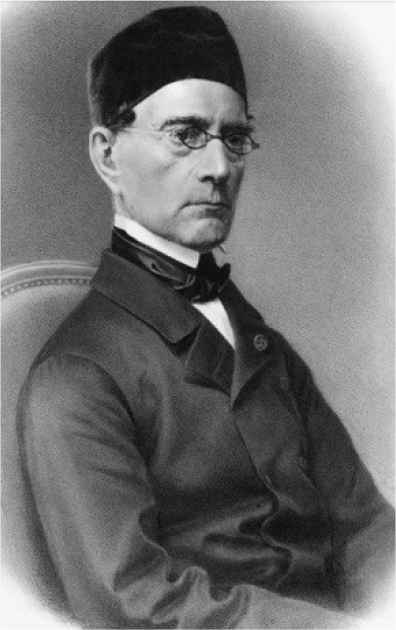
Gabriel Lamé.
5.3. Building Bridges
Lamé curves became well known as supercircles in the second half of the 20th century through the work of Danish mathematician, inventor and poet Piet Hein (1905–1996) [22]. Sergel’s Torg in Stockholm (Fig. 12) is modeled as a superellipse. Later, Piet Hein designed lamps, beverage coolers, tableware and tables based on superellipses and the 3D forms he called supereggs (Fig. 12). The superegg has a circular cross-section in one plane and a supercircular cross-section in the perpendicular plane. There are many other examples of supercircles and superellipsoids in architecture, and in computer graphics superellipsoids and superquadrics are well known [25]. As shown above, they have a long and very interesting history. These remarks on the history of geometry serve as introductory remarks aimed at establishing a coherent framework. The goal of this framework is a unification of geometry based on ancient principles and supported by our observations of natural forms and phenomena.
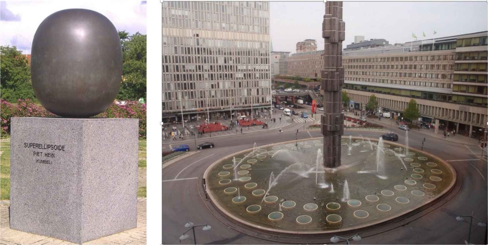
Superegg (left) and Sergel’s Torg (right) in Stockholm, Sweden.
5.4. Building Bridges in Space and Time
We find the footprint of Lamé everywhere and the generalization to Gielis Transformations provides more flexibility, including symmetry. Fig. 13 shows starfishes from four different genera [53]. One may imagine that these starfish could be different individuals or different ecotypes of one species, or morphological changes during their evolution from small to large with increasing elongation of the arms. In the first case, their different sets of parameters could lead to classifications. In the second case, we have the evolution from a small starfish to an adult starfish; in this case, the change in parameters has a direct relevance to the evolution of the individual.
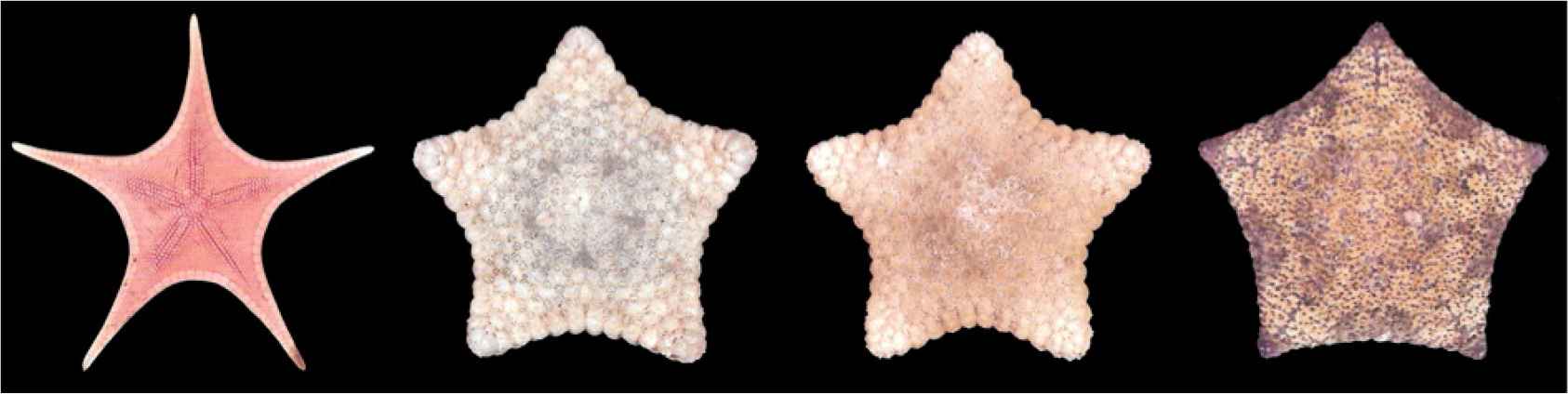
Various starfish [46].
Modeling a variety of natural shapes and phenomena, such as leaves, seeds, starfish, diatoms [59], square bacteria [60], superelliptical galaxies [61] or even snowflakes [5], can now be done in one coherent framework as a complete scientific methodology. Lamé curves and Gielis Transformations now also have a place in geometry [62], mathematics [63] and physics based on minimization principles [49].
One example of such minimizing principle is provided by tree rings. Lamé curves may be considered as a generalized Pythagorean Theorem with conservation of n-surfaces (of which area and volume are only two examples). In the case of power laws, one has
It is interesting to see how nature “computes” shape and optimization. Lamé curves and Gielis Transformations are non-linear, but if one considers the formation of a tree ring [48] as the result of both evolutionary and developmental processes, dealing with biotic (insects, fungi, viruses) and abiotic (light, temperature, rainfall, soil, frost, etc.) influences and stresses at very different time scales, it is at least remarkable that the resulting shapes are described by superellipses with exponent
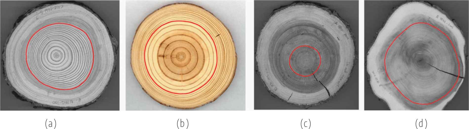
Superelliptical tree rings in softwoods: (a) Jack pine (Pinus banksiana); (b) red pine (Pinus resinosa); (c) tamarack (Larix laricinia); (d) white cedar (Thuja occidentalis) [48].
5.5. A Geometrical Language for the Unique
This article focused on five central themes.
First, a unified view leads to a strong reduction of complexity, especially with respect to mathematics as the language of the sciences. This unification combines power laws, Lamé curves, distance measures and functions, and geometries, into a single framework. I named this after Gabriel Lamé, who was the first to systematically study higher-order curves in two variables, which have become known as Lamé curves. Extending Lamé curves to Gielis Transformations provides for a new but sound scientific methodology which has been tested on more than 40,000 biological specimens. It turns out that circles and ellipses are very rare in nature, whereas supercircles and superellipses are very common.
Second, this unified view traces back to the very foundations of mathematics and geometry as generalizations of the methods laid down in Ancient Greek geometry. Power laws, superellipses and Gielis Transformations are simply variations on a single theme. Using addition or multiplication, we obtain simple generalizations of the Pythagorean Theorem and the classical means (geometric, arithmetic and harmonic) which led to the classical conic sections. Many of the existing methods in mathematics suffice [5,63]. Obviously, power laws have been used as a scientific methodology for many decades. A single generalization of the conic sections encompasses such a wide variety of natural and abstract shapes, as a continuous transformation, that the notion of complexity of shapes needs to be revisited [5].
Third, what is improbable in our current scientific views, e.g. 50 heads or tails in a row, turns out to be the essence of natural shapes and forms. Nature likes biased coins. However, the improbable and the most probable co-exist in natural systems. In one and the same system, high and low entropy balance each other. For example, the high information content in the genetic code is effectively protected by the double-stranded nature of DNA.
Fourth, each shape can have its own parameters that distinguish it from every other shape, however large or small. These parameters may change over time and the smallest variation of all forms tested can be quantified with any desired precision. Any single variation in starfish or along the stems of square bamboo or softwood trees, diatoms, bacteria or galaxies can be uniquely quantified. Unique leaves acquire unique parameters and this can be extended to a wide range of natural forms, including diatoms, bacteria and galaxies. This can be extended to the great and the small.
Mathematics has a chance – at last – of also becoming the science of the individual; the same individual that played no role in science so far. Science has become successful by reducing objects (and subjects) to just a few characteristics. In the extreme, quantum mechanics and thermodynamics are built upon the criterion of indistinguishability, in which individuality is effectively obscured. Understanding that mathematics is not only the language of patterns, developing mathematics as the language for the individual is a key component of future science and knowledge.
Finally, it is enlightening to find that it is a simple combination of individual monomials, either by addition or multiplication, which provides us with a number of key methods for studying natural forms and phenomena from a common and individual perspective. In the case of DNA, we see a maximum entropy for single strands and a minimum entropy for double-stranded molecules. The highest and the lowest of the possible values. The attentive reader will have noticed that for
Unity in Multiplicity and Diversity from Unity… Inspired by Gabriel Lamé (Saint-Gabriel is also one of the Archangels, bearer of divine messages and inspirations!), these new insights open new doors and will allow us to continue climbing and, hopefully and finally, conquering Mount Improbable.
Footnotes
“Useful energy” is somewhat anthropocentric, in the sense of “usefulness for humans”.
Obviously, there is no reason to stop at the fourth row.
Lamé curves have the same exponent for each parameter. Euzet generalized this some decades later.
No need for new rules, just stick with old wisdom.
Modular or clock arithmetic.
Note that such laws are not absolute, but relative to the conditions such as temperature for living organisms.
REFERENCES
Cite This Article
TY  - CONF
AU  - Johan Gielis
PY  - 2023
DA  - 2023/11/29
TI  - Conquering Mount Improbable
BT  - Proceedings of the 1st International Symposium on Square Bamboos and the Geometree (ISSBG 2022)
PB  - Athena Publishing
SP  - 153
EP  - 174
SN  - 2949-9429
UR  - https://doi.org/10.55060/s.atmps.231115.013
DO  - https://doi.org/10.55060/s.atmps.231115.013
ID  - Gielis2023
ER  -


