
From Pythagoras to Fourier and From Geometry to Nature
DOI: https://doi.org/10.55060/b.p2fg2n.ch009.220215.012
Chapter 9. From Lamé Curves to Gielis Transformations
9.1 Riemann’s Geometric Ideas
In the mid-19th century geometry went multidimensional when Riemann defined analytically n-fold extended manifolds, where each point can be described by an n-tuple of numbers (their coordinates). Following Gauss’ work on surfaces embedded in E3 he also used systems of local coordinates, as a relevant extension of the geometry of surfaces in Euclidean space E3 based on the Pythagorean theorem [61]. In his famous memoir, Riemann explicitly mentioned the geometric tangent 2 − D indicatrix of fourth order x4 + y4 = 1 as an extension of the Euclidean circle x2 + y2 = 1. He thus conceived of distance metrics (9.1) [47]:
With the Euclidean distance for p = 2, this forms a bridge between classical Euclidean geometry and Riemannian geometry (with a “quadratic” distance form based on Pythagoras) on the one hand, and Finsler geometry (“without the quadratic restriction”) and metric spaces (“with the m-th root metric”) on the other [30]. In the infinitesimal form (9.1) the simplest so-called Riemann-Finsler geometries are defined [47]. These also find applications beyond geometry. For example, in the early 1990s P.L. Antonelli proposed a Lamé metric in ecology [2]:
Equation (9.1) can account for any number of dimensions, for example, defining Minkowski distances in Lp spaces [83]:
These types of equations are systematically discussed for the first time in a booklet Examen des Différentes Méthodes Employées pour Résoudre les Problèmes de Géométrie, published in 1818 by Gabriel Lamé [66]:
These equations describe the so-called one-parameter Lamé curves (Figure 19). Since a circle is defined in a plane by a total of three numbers (the coordinates of its center and its radius), the totality of all circles in the plane is a 3-dimensional manifold. The totality of all ellipses in the plane is a 5-dimensional manifold with the major and minor axes and orientation of the ellipses [61].
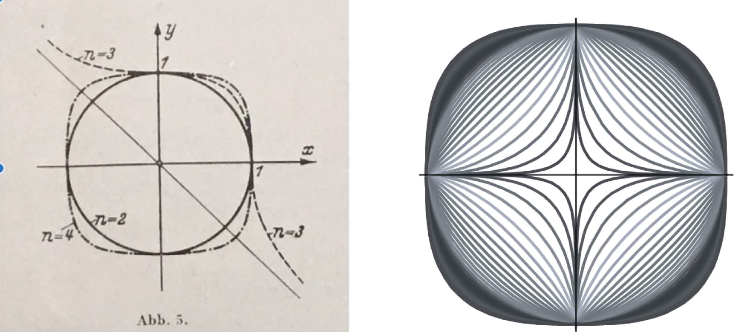
Left: Lamé curves for odd and even exponent values [53]. Right: supercircles, also for n < 2.
However, all Lamé curves defined by (9.4), which includes all circles, all squares (the inscribed squares for n = 1 and the circumscribing squares for n → ∞), all astroids (for n = 2/3), as well as all supercircles for any n > 0 (Equation 9.5a), still constitute only a 4-dimensional manifold, or a 5-dimensional manifold for superellipses (Equation 9.5b). Gielis curves are a relevant extension of Lamé curves adding a few more parameters. These curves and transformations provide for a unified description of natural shapes [47]. In Part IV many examples are shown.
9.2 Lamé Curves and Superellipses
In a Cartesian (x, y) system, Equation (9.4) (with n a positive integer which Lamé assumed > 1) defines the so-called Lamé curves with base radius R. For even n, the curve (9.4) is a closed curve without real double and inflection points and with the four symmetry axes x = 0, y = 0, x = ±y. For odd n, it is a single curve without real double point, with the two inflection points (1; 0) and (0; 1), the symmetry axis x = y and the asymptote x = −y (Figure 19) [53]. Supercircles or superellipses, both a subset of Lamé curves and a generalization of the circle, are based on Equations (9.5a) and (9.5b) with n a positive integer and using absolute values to ensure that shapes are closed.
In fact, many problems of analytic geometry that have become part of modern geometric techniques and textbooks were first solved by Gabriel Lamé. Here we find the first mention of the equation of a plane in the form
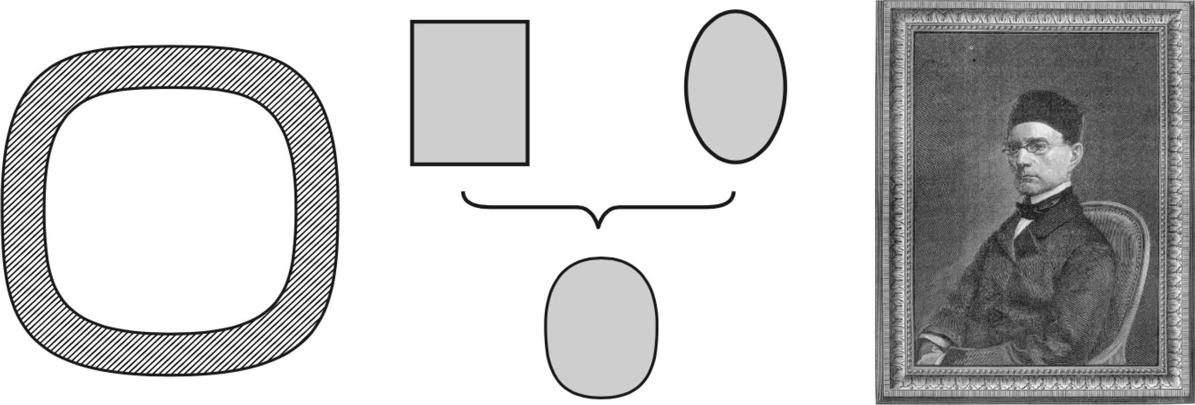
Left: superelliptical section of a square bamboo. Center: optimal solution according to Piet Hein. Right: Gabriel Lamé [41].
Gabriel Lamé (1795–1870) attended the École Polytechnique in Paris from 1813 to 1818 and graduated from the School of Mines in 1820. Over the next decade, from 1820 to 1831, Lamé worked in Saint-Petersburg responsible for railways and bridges [51]. After returning to Paris, Lamé became Professor of Physics at the École Polytechnique. Lamé’s mathematical discoveries are closely linked to his research on the theory of elasticity. He is considered a father of mathematical physics with the introduction of the parameters (invariants) of a scalar field of first and second kind [41].
Δ2F and Δu are the Laplacian, expressed in Cartesian and polar coordinates respectively. The curvilinear coordinates and the differential parameters introduced by Lamé inspired the Italian school of differential geometry with Ricci, Levi-Civita and Beltrami. Gabriel Lamé should not only be considered as one of the founders of differential geometry, but also of Riemannian geometry in the opinion of Elie Cartan (1869–1951) who was a leading geometer of the 20th century [55]. He was the first to apply curvilinear coordinates in space using an orthogonal system, giving the length of an element as:
He was naturally led to Fermat’s Last Theorem since this is exactly Equation (9.5a) and he proved the case for n = 7. The recurrence formula that gives rise to Fibonacci numbers was used by Lamé to develop the Euclidean algorithm, to determine the greatest common divisor of two integers [69], and is still in use today. Gaston Darboux spoke of the immortal works of Gabriel Lamé and Gauss called him the best French mathematician of his time. On the Eiffel Tower, the names of Fourier, Carnot and Lamé are very close together, all on the Bourdonnais side of the Tower.
Due to the work of the Danish mathematician and inventor Piet Hein, Lamé curves became very popular in the 1960s, in objets d’art, furniture, pottery, fabric patterns, etc. But his major achievement to date is a sunken oval shopping plaza, promenade and pool in the center of Stockholm. For Piet Hein the superellipse was an iconic solution between a round and a square worldview: “Man is the animal that draws lines, which he himself then stumbles over. In the whole pattern of civilization there have been two tendencies, one toward straight lines and rectangular patterns and one toward circular lines. There are reasons, mechanical and psychological, for both tendencies. Things made with straight lines fit well together and save space. And we can move easily - physically or mentally - around things made with round lines. But we are in a straitjacket, having to accept one or the other, when often some intermediate form would be better. To draw something freehand - such as the patchwork traffic circle they tried in Stockholm - will not do. It isn’t fixed, it isn’t definite like a circle or square. You don’t know what it is. It is not esthetically satisfying. The superellipse solved the problem. It is neither round nor rectangular, but in between. Yet it is fixed, it is definite - it has a unity. The superellipse has the same beautiful unity as the circle and ellipse but is less obvious and less plain. The superellipse frees us from the straitjacket of simple curves such as lines and planes.” [42]
9.3 Trigonometry of Supercircles and a Generalization of π
The sector of area bounded by the curve between the positive x-axis and the driving ray from the zero point to the point of the curve (x, y) (Figure 21) is denoted by (1/2)ν, because in the case of n = 2 of the circle it is half the central angle of the sector. Its double value is [53]:
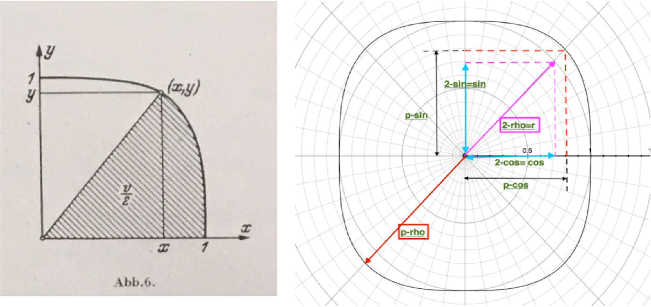
Left: sector of superellipse [53]. Right: trigonometric functions on a supercircle.
Depending on whether the expression is of y in x, or of x in y according to (9.5b), the first or the second of the following integrals is obtained:
These integrals are denoted by arccosn (x) and arcsinn (y) and their inverse functions by cosn ν and sinn ν, thus:
These integrals pass into the functions arccos(x) and arcsin(y) for n = 2. The functions tann ν and cotannν are defined by:
This leads to the natural generalization in the system ẋ = yp, ẏ = −xp, of the differential equation system ẋ = y, ẏ = −x. Combining (9.4) right (the unit circle) and (9.9a)–(9.9b) it follows that [53]:
These are the differential equations for the functions sinn ν and cosn ν, namely:
Furthermore, it follows according to (9.12):
Hence the functions cosn ν and sinn ν both obey the differential equation:
For each supercircle one can define the perimeter as 2πn. To determine the half-perimeter πn we can use the integral value [53]:
One finds the values shown in Table 1 and, according to the geometric meaning, one supposes the limit π∞ = 4. To confirm this, one introduces the Gamma function which gives:
| n | πn |
|---|---|
| 2 | 3.142 |
| 3 | 3.533 |
| 4 | 3.708 |
| 5 | 3.801 |
| 6 | 3.855 |
| 7 | 3.890 |
| 8 | 3.914 |
| 9 | 3.931 |
| 10 | 3.943 |
| ∞ | 4.000 |
See [51].
Unit supercircles thus have dedicated trigonometric functions [42, 53, 67] and a dedicated value of πn, defined as the half-perimeter of the super- (or sub-)circle with exponent n (Figure 21 and Table 1) [67].
For n = 2 the functions cosn(ϑ) = cos(ϑ) and sinn(ϑ) = sin(ϑ), and additionally tann(ϑ) = tan(ϑ). This gives the generalized Pythagorean theorem:
9.4 From Superellipses to Gielis Transformations
Using ρ = R cos(ϑ) and ρ = R sin(ϑ) and using different exponents n1, n2, n3 gives [7, 40, 92]:
And for the superellipse with semi-major and semi-minor axes A, B:
The restriction to the Cartesian coordinate system is solved by adding a symmetry parameter
Examples are shown in Figure 22 (a) to (f) [40]. More generally, Equation (9.23) can be a transformation of any planar function f(ϑ):
Examples of transformations of spirals and trigonometric functions are shown in Figure 22 (g) to (i) and Figure 22 (j) to (l) respectively; see also [46, 56, 90].
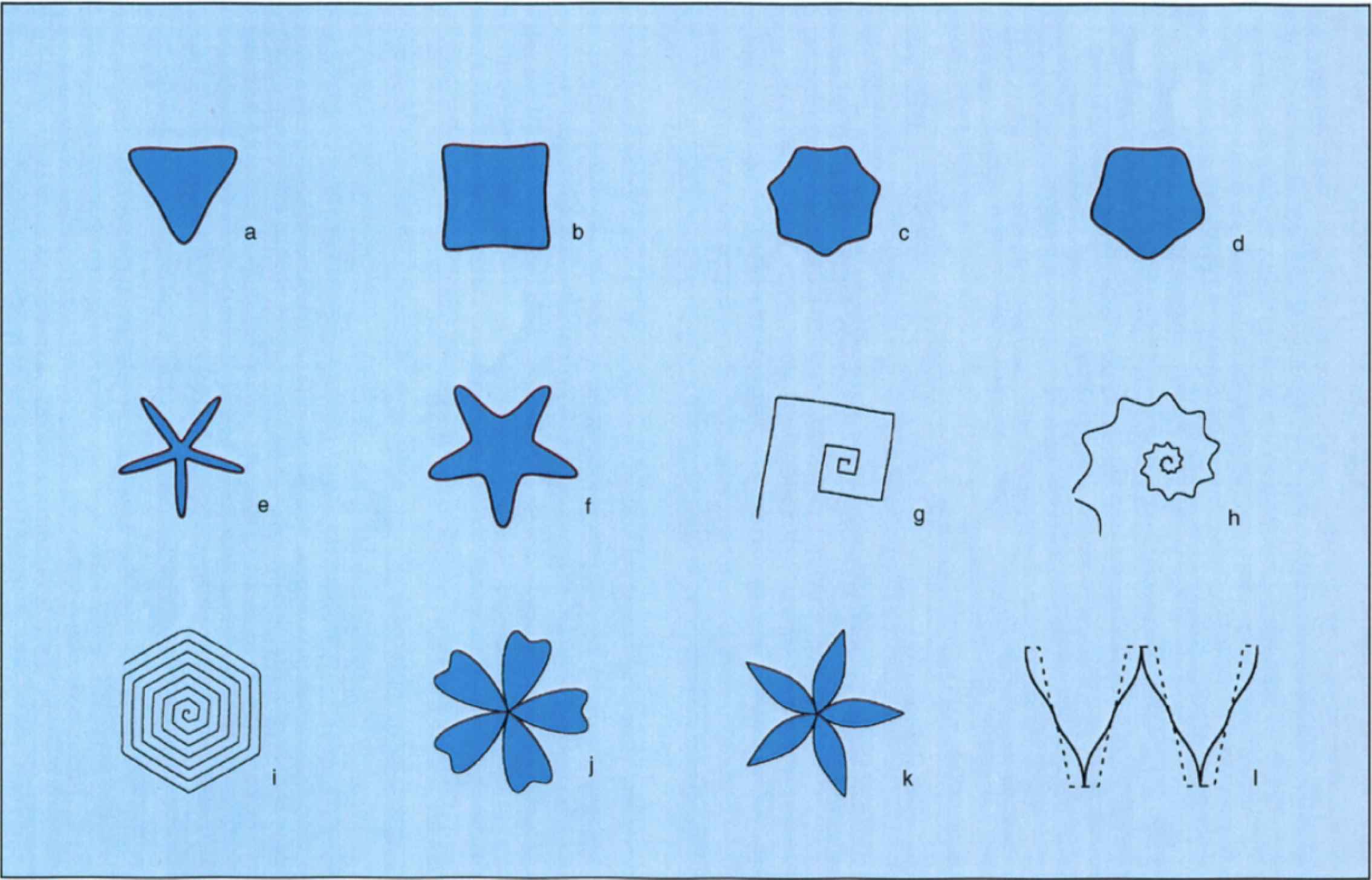
(a)–(d): cross sections of plant stems. (e)–(f): starfish. (g)–(i): transformations of logarithmic (g+h) and Archimedean (i) spirals. (j)–(l): transformations of cosines, as flowers or in wave view [40].
The symmetry parameter m can be integer, rational or irrational (Figure 23). Rational values of m generate polygrams. Regular m-polygons are defined as [14]:
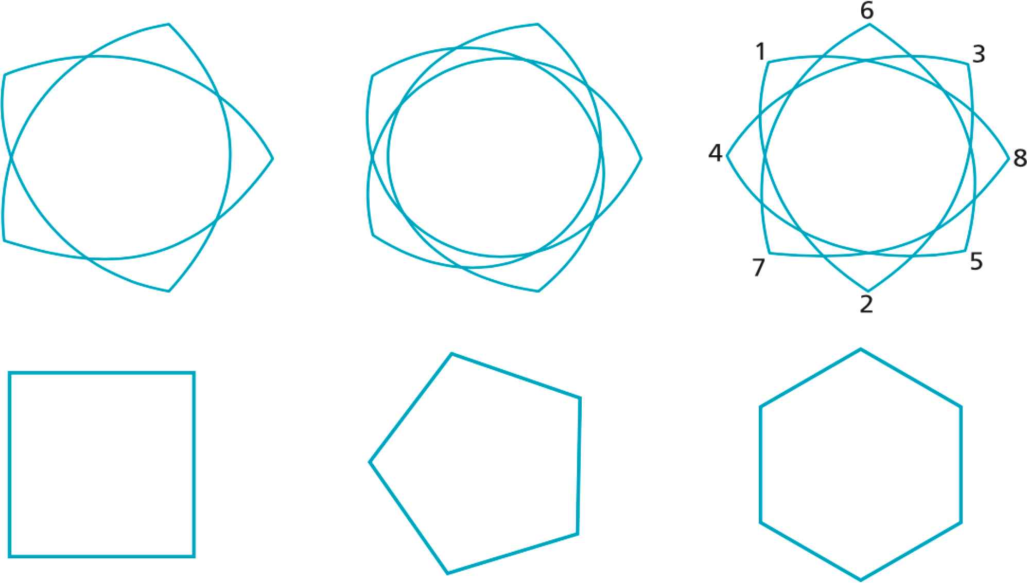
Top row: self-intersecting polygons for
Examples are shown in Figure 23 bottom row. Approximations to regular polygons and polygrams are obtained by defining regular Gielis polygons [72]:
For m > 5, the deviations of Gm,n2,3,n1 from true regular polygons are less than 1%, monotonically decreasing for increasing m [72].
Using Equation (9.23) as equality:
The inequality:
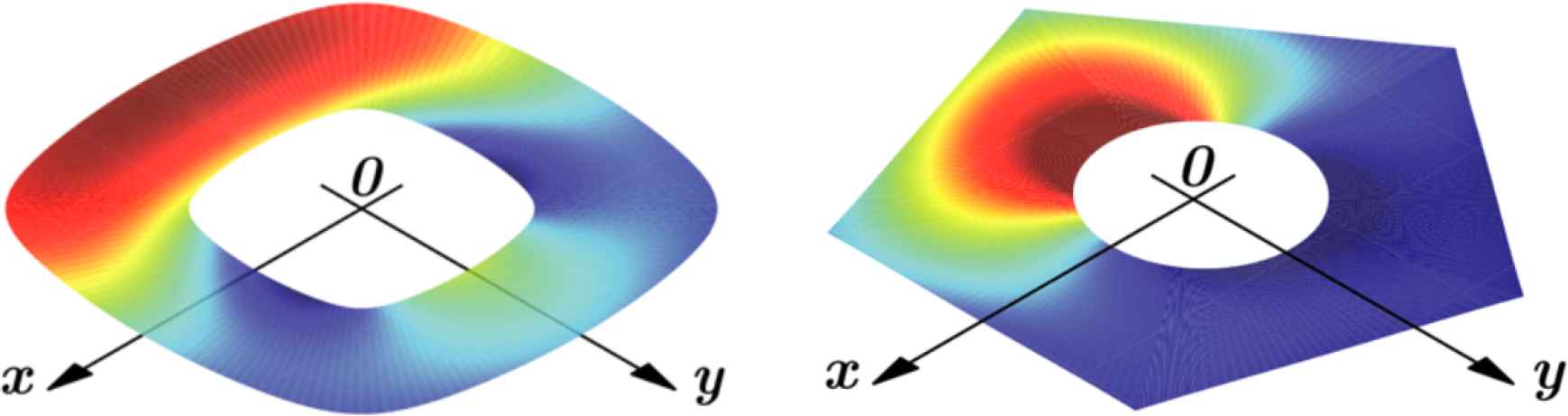
Annuli with same or different outside and inside boundaries. On the right the outer boundary is a regular pentagon. [14]
9.5 Generalizations
R. Chacón proposed the following equation [25]:
Here ϑ ∈ [−π, π]; f1, f2 and c(ϑ) are continuous functions; m1, m2, A, B, n1,2,3 are real numbers; and A, B, n1 are not zero. Division by 4 in the preceding formula is unnecessary of course, since the same results can be simply obtained by changing the values m1 and m2. Actually, this division is only assumed in order to preserve the original form of the Gielis Superformula and the special case of Lamé curves for m = 4. It is then possible to impose conditions, such as conditions for functions to be increasing f(−π) = −π, f(π) = π, closed f(−π) = f (π), or to pass through the origin [48]. Some further examples are shown in Figure 25.
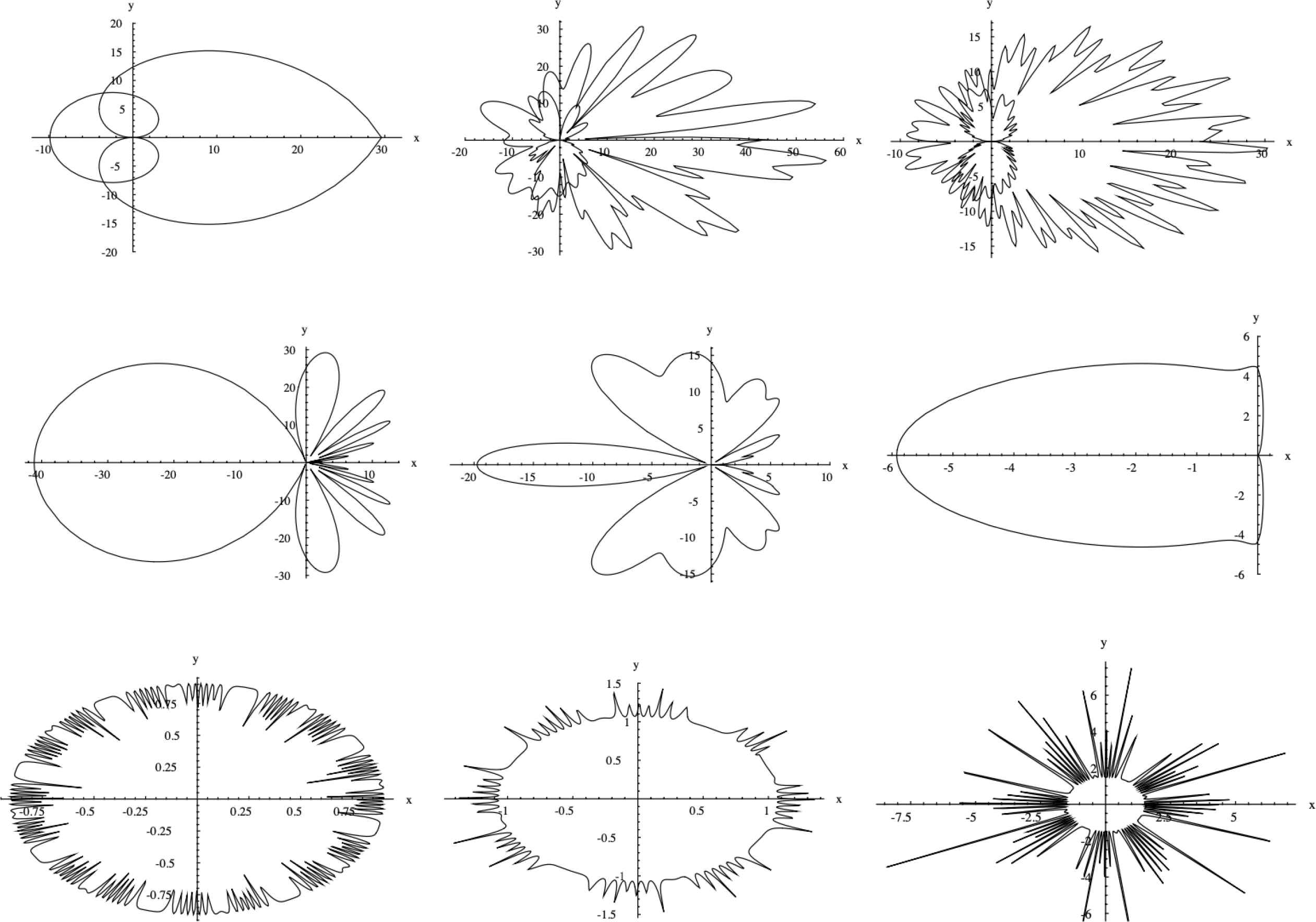
Examples of generalized Gielis transformations [48].
9.6 Supercircles and Superparabolas
The structural form of the above equations is both Pythagorean-compact and topologically simple. The basic structure is [41]:
| Variables | Planar curves | Types | Special means |
|---|---|---|---|
| xn + yn | Supercircles & Superellipses | Lamé curves | Arithmetic mean |
| xn ⋅ ym | Superparabolas & Superhyperbolas | Power laws | Square of geometric mean |
Lamé curves and power laws as generalizations of conic sections [46].
In the same way as supercircles are generalizations of circles, these power relations are superparabolas which are generalizations of the classic parabola y = x2. In Figure 26 left, superparabolas y = xn/m are shown in the interval [0; 1] and the exponents range from n = 1/2 to n = 2 with steps of 1/5. The cases for n > 1 and n < 1 have y = x with n = 1 as the symmetry axis (the bisectrix). The classic parabola is a machine that turns a rectangle with area y ⋅ 1 into a square with the same area and side x, which is the geometric mean. In the same way, a superparabola y = xn/m turns a beam with an n-volume into a cube with an m-volume (for n < m) [41].
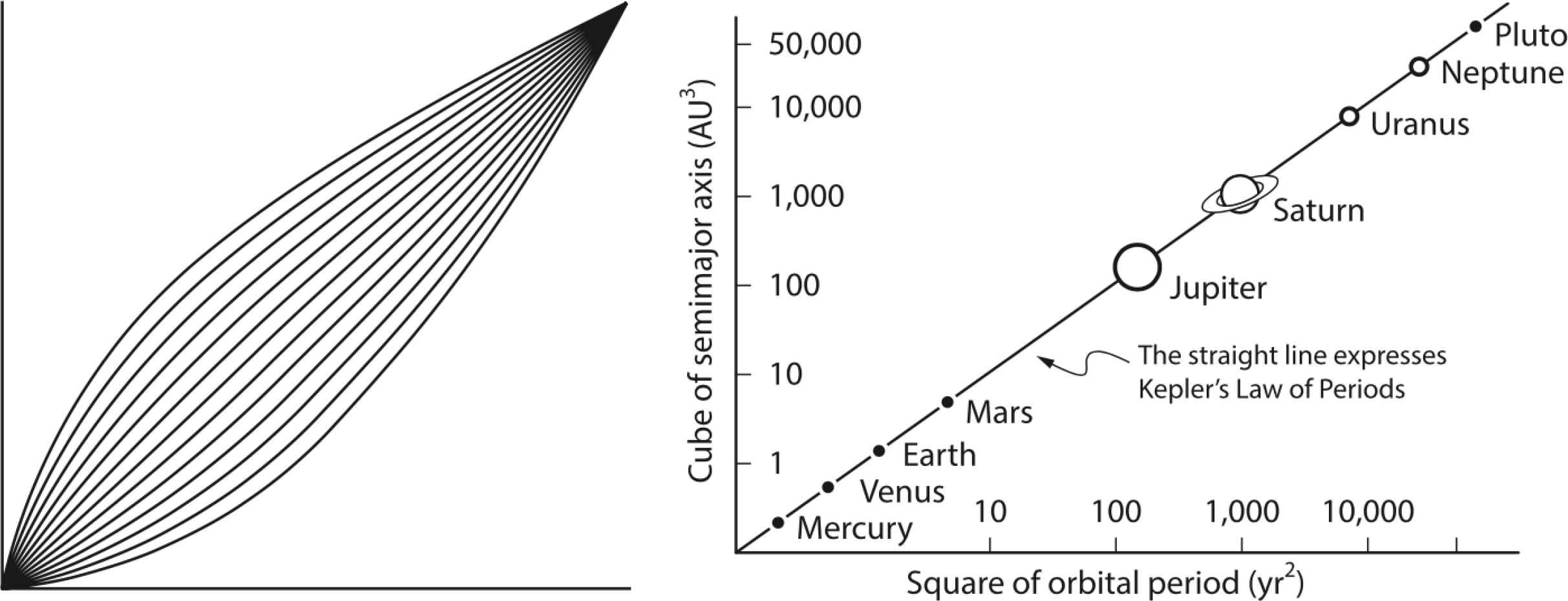
Left: sub- and superparabolas in the interval [0; 1]. Right: Kepler’s Law [41].
The trigonometry of the parabola yields interesting insights. The value of the half-perimeter πpar is a rational number and is directly related to Archimedes’ Quadrature of the Parabola. Moreover, the values of the associated secpar and cospar at 45° give the Golden Ratio φ and its inverse 1/φ respectively [32, 33, 91]. The generalization of these trigonometric functions to super- and subparabola, analogous to the trigonometry on supercircles, needs to be developed.
In physics, biology and economy, power laws are found everywhere, from the size of cities to the power noise in time series. The Cobb-Douglas production function V = γKδL1−δ is one example from economics, with the output of a Process V defined by Capital K and Labor L, which can be substituted to a certain extent depending on the substitution parameter δ. This is equivalent to an expression like z = xn ⋅ ym. In the case of Cobb-Douglas n = 1−m. Actually, the Cobb-Douglas model is a limiting case of the CES (constant elasticity of substitution) production models (in the case of ρ = 0 elasticity reduces to unity) [3]:
For more information, please contact us at:
info@athena-publishing.com


