
From Pythagoras to Fourier and From Geometry to Nature
DOI: https://doi.org/10.55060/b.p2fg2n.ch015.220215.018
Chapter 15. Trigonometry on the Diamond
The approximation of any function to any desired precision with a sum or series of sines and cosines via Fourier series expansions is a wonderful mathematical tool which is widely used in technology and science, either on time series or closed shapes such as plant leaves. We already know that on each supercircle and superellipse we can define a specific Pythagorean theorem with associated trigonometrical functions.
Now what if our time-series is a collection of discrete measurements connected via lines? Such piecewise linear graphs occur, for example, in seismic measurements or sampling of sounds. In the conversion of analog sound to digital, samples are taken at specified intervals and from this the digital signal is constructed. What if we can consider such series as connected points of a piecewise-linear graph rather than approximate them with sinusoidal functions?
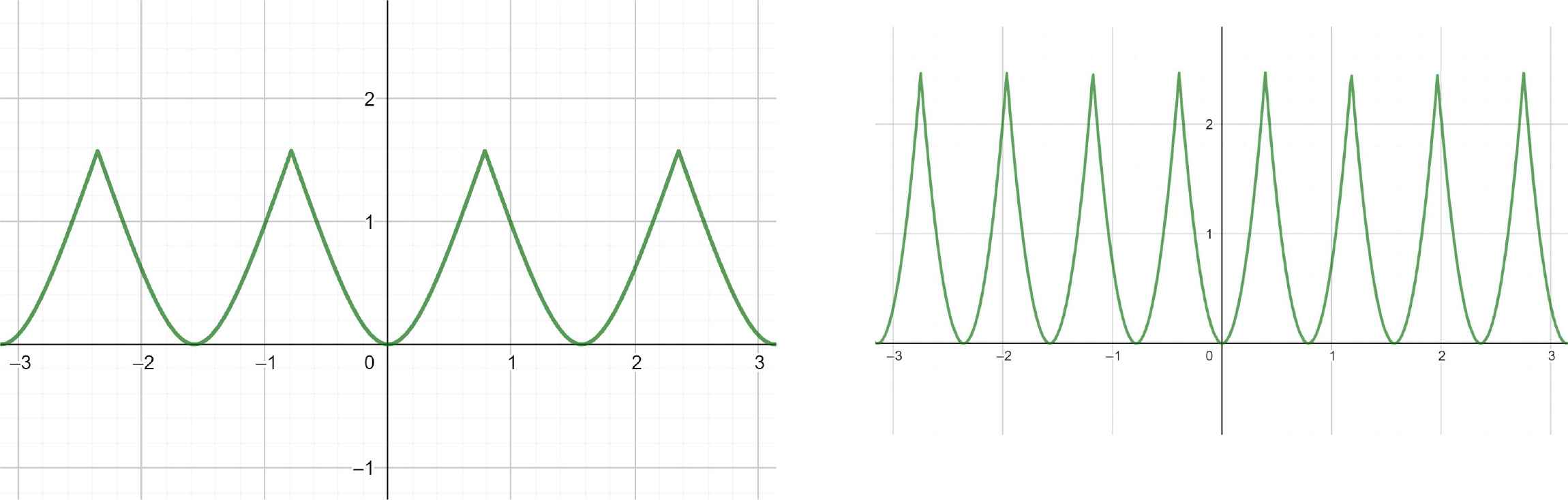
It turns out that this can be done using inverse trigonometric functions [78]. The diamond, a subellipse with exponent n = 1, can be described by x = arcsin(cos t) and y = arcsin(sin t) (Figure 69 left), and the corresponding trigonometric functions are defined immediately (Figure 69 right). The graphs in Figure 70 show the Lissajous figures with x = arcsin(cos(At)) and y = arcsin(sin(Bt)) for particular values of A and B. For any A = B we recover the diamond. One can construct polynomials as sums (Figures 71 and 72).
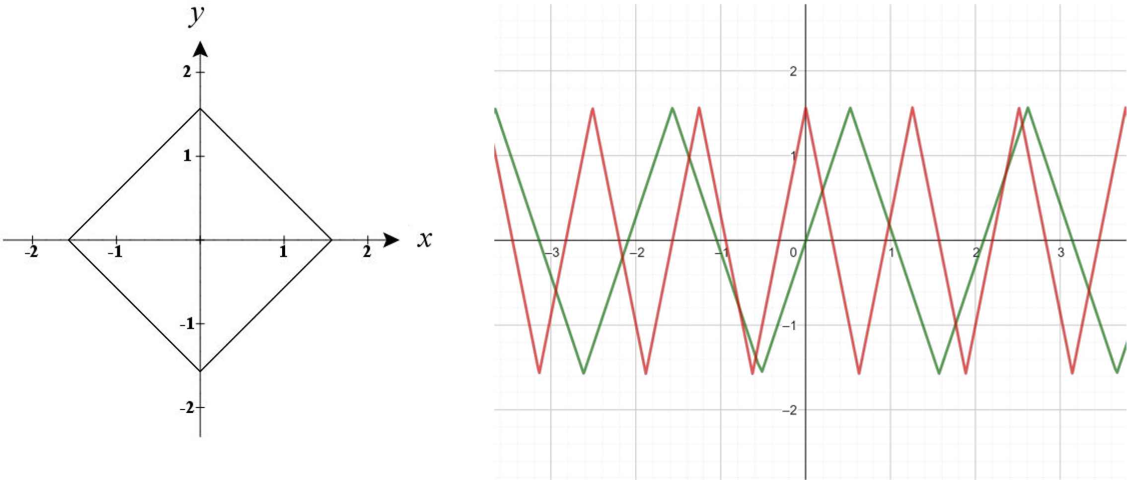
Left: the diamond. Right: arcsin(sin(3t)) (green) and arcsin(cos(5t)) (red).
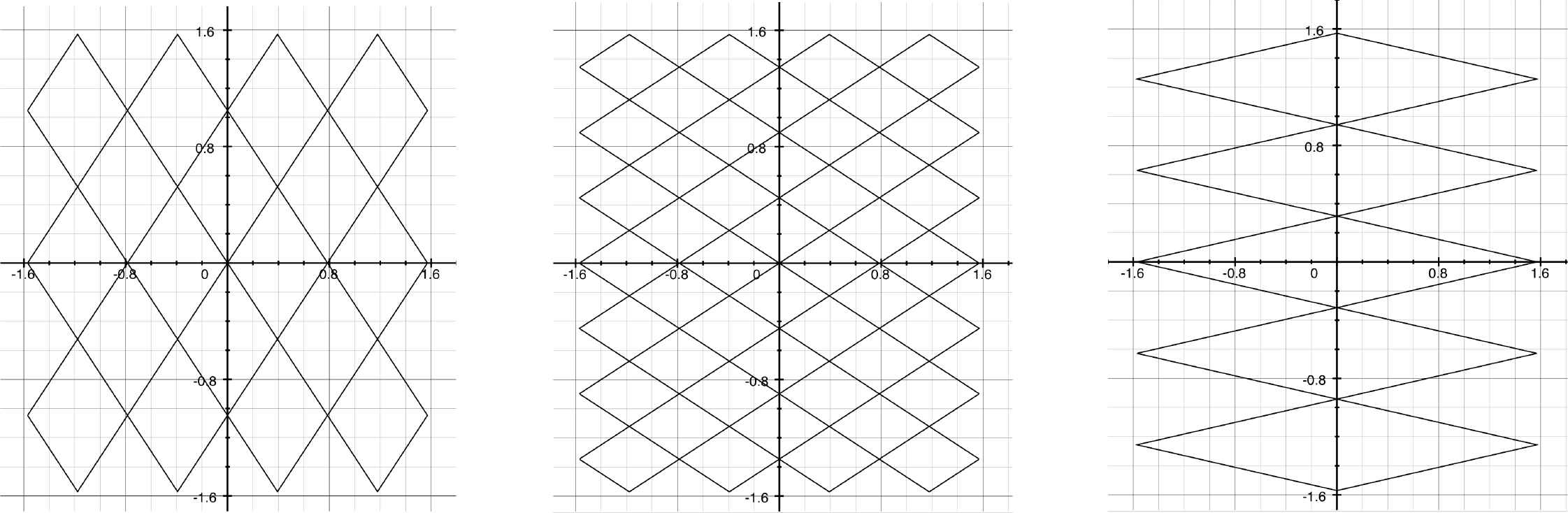
Lissajous figures with x = arcsin(cos(At)) and y = arcsin(sin(Bt)). Left: A = 3, B = 4. Center: A = 7, B = 4. Right: A = 5, B = 1.
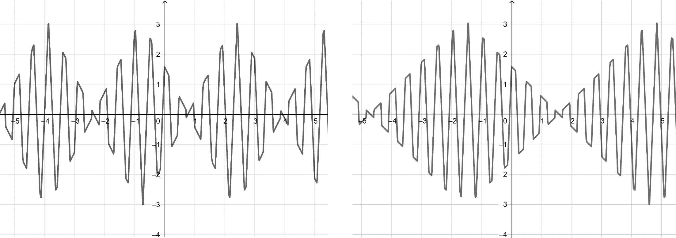
Left: arcsin(sin(11t)) + arcsin(cos(13t)). Right: arcsin(sin(12t)) + arcsin(cos(13t)).
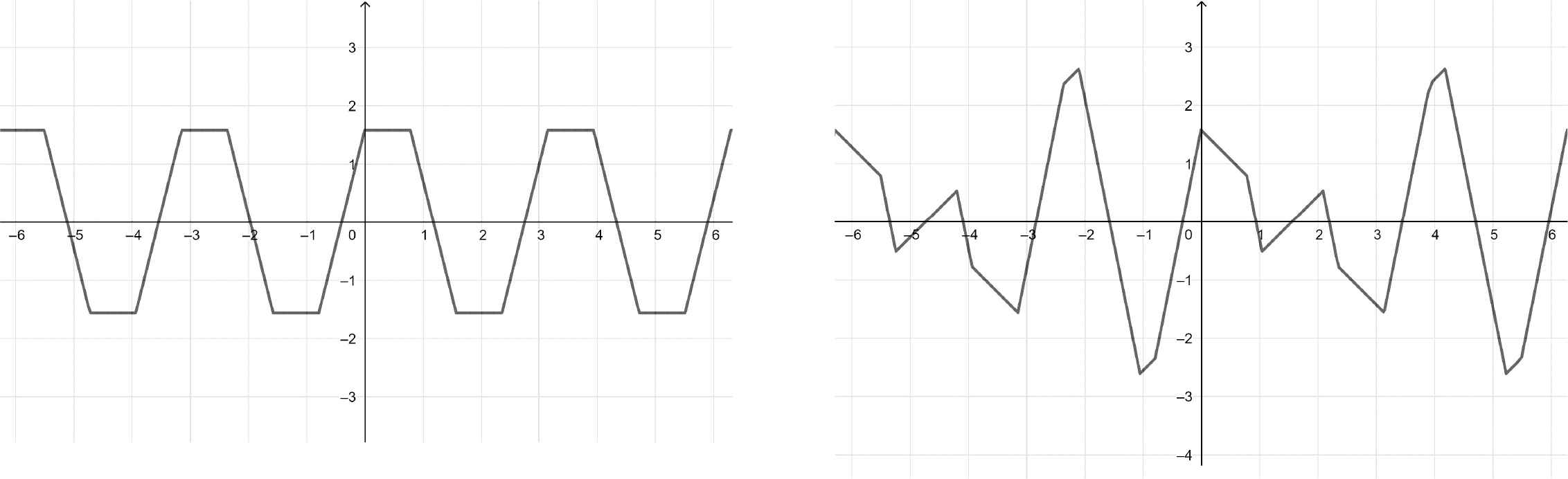
Left: arcsin(sin(2t)) + arcsin(cos(2t)). Right: arcsin(sin(2t)) + arcsin(cos(3t)).
15.1 D-Fourier Polynomial Expansions
As it seems that only a small number of D-trigonometric functions are sufficient to approximate graphs of complicated shapes, in what follows we consider only D-Fourier polynomial expansions, avoiding the complicated problems of series’ convergence.
Given a function f(t) ∈ L2(π, π), put:
The integrals in the denominators of Equations (15.5) and (15.6) are given by:
Then, introducing the constant D ≔ 5.16771... we find:
Therefore, Equation (15.1) writes as:
In Figure 73, the graphs of the functions arcsin(sin(2x))2 (left) and arcsin(sin(4x))2 (right) are shown.
Left: arcsin(sin(2x))2. Right: arcsin(sin(4x))2.
Hence, the analogues of circular functions are defined and formulas are constructed that translate the trigonometric ones. The relative D-trigonometric functions have geometric shapes closely related to the corresponding classical ones. For these functions, the orthogonality property has been proven and finite combinations of D-trigonometric functions allow to write the piece-wise linear functions in a simpler way with respect to their Fourier expansions. Possible applications can be found in the representation of sounds or seismic waves generated by earthquakes.
15.2 Nature: An Endless Source of Inspiration
The application of mathematics to physical and natural phenomena in almost all cases makes use of pre-existing mathematical structures, such as Riemannian geometry and tensor calculus for general relativity, and matrices and Hilbert spaces for quantum mechanics. According to René Thom (Fields Medal 1958): “There is only one authentic counterexample to the thesis supporting the preformed, almost a priori character of the mathematical structures applied progressively to theoretical physics or to other branches of knowledge of reality: Fourier’s wave theory. It is very clear that the Fourier series theory was really inspired by physics, more precisely by the study of vibrating strings or the theory of heat.” [98]
Gielis curves were inspired by botany and various symmetries in nature, expanding Gabriel Lamé’s proposed use of superellipses to model crystals to a very wide range of natural shapes and phenomena. This is a second example of a mathematical development inspired by natural shapes and phenomena. Indeed, the profound study of nature is the most fertile source of mathematical discoveries, as Fourier wrote.
In this book, these two methods have been combined by showing how the original Fourier projection method can be used to solve boundary value problems on normal polar domains, in particular Gielis domains. Moreover, since each specific instance or curve comes with its proper trigonometric functions and Pythagorean theorem, this opens up new possibilities and connections in mathematics. In specific cases like the diamond, this leads to generalizations of Fourier’s work to deal with piecewise linear functions.
For more information, please contact us at:
info@athena-publishing.com


