
Revised 21 July 2023
Accepted 9 October 2023
Available Online 29 November 2023
- DOI
- https://doi.org/10.55060/s.atmps.231115.010
- Keywords
- EWQPSO algorithm
Antenna design
Superformula - Abstract
Electromagnetic design problems involve optimizing multiple parameters that are nonlinearly related to objective functions. Traditional optimization techniques require significant computational resources that grow exponentially as the problem size increases. Therefore, a method that can produce good results with moderate memory and computational resources is desirable. Bioinspired optimization methods, such as particle swarm optimization (PSO), are known for their computational efficiency and are commonly used in various scientific and technological fields. In this article we explore the potential of advanced PSO-based algorithms to tackle challenging electromagnetic design and analysis problems faced in real-life applications. It provides a detailed comparison between conventional PSO and its quantum-inspired version regarding accuracy and computational costs. Additionally, theoretical insights on convergence issues and sensitivity analysis on parameters influencing the stochastic process are reported. The utilization of a novel quantum PSO-based algorithm in advanced scenarios, such as reconfigurable and shaped lens antenna synthesis, is illustrated. The hybrid modeling approach, based on the unified geometrical description enabled by the Gielis Transformation, is applied in combination with a suitable quantum PSO-based algorithm, along with a geometrical tube tracing and physical optics technique for solving the inverse problem aimed at identifying the geometrical parameters that yield optimal antenna performance.
- Copyright
- © 2023 The Authors. Published by Athena International Publishing B.V.
- Open Access
- This is an open access article distributed under the CC BY-NC 4.0 license (https://creativecommons.org/licenses/by-nc/4.0/).
1. INTRODUCTION
Optimization is a widely used concept in many fields, such as engineering, economics, management, physical sciences, and social sciences. Its purpose is to identify the global maximum or minimum of a fitness function. Finding all optimal points of an objective function can aid in selecting a robust design that simultaneously considers various constraints and performance criteria.
Designers of microwave and antenna systems face the challenge of finding optimal solutions for electromagnetic problems of increasing complexity. This can be a difficult task as it involves evaluating electromagnetic fields in three dimensions, considering a large number of parameters and complex constraints, and dealing with non-differentiable and discontinuous regions. These optimization problems are often non-linear and more challenging to solve than linear ones, especially when many locally optimal solutions are in the feasible region.
When developing electromagnetic systems, it is essential to carefully consider how the different design elements interact with each other. Instead of relying on brute-force computational techniques, experts use advanced optimization procedures to achieve the best results. These procedures can be grouped into two categories: deterministic and stochastic methods. While deterministic methods have their advantages, stochastic methods have the potential to find the global optima of a problem, no matter where the search begins. Stochastic algorithms are highly valued by electromagnetic engineers for their ability to efficiently find global optima, even when faced with nonlinear and discontinuous problems that involve many variables. They are flexible, adaptable, easy to implement, and can handle complex fitness functions without requiring the computation of derivatives. Unlike traditional searching methods, these algorithms are not overly reliant on the starting point, making them an invaluable tool for optimizing non-differentiable cost functions in complex multimodal search spaces. However, due to their stochastic behavior, these algorithms require many iterations to produce reliable results.
Various swarm intelligence-based optimization algorithms have been developed to address the differing descriptors and unknowns in each optimization problem. These algorithms include particle swarm optimization, ant colony optimization, cuckoo search, firefly algorithm, bat algorithm, artificial fish swarm algorithm, flower pollination algorithm, artificial bee colony, wolf search algorithm, and gray wolf optimization [1]. Choosing the most suitable algorithm is crucial, as there is no general rule for this decision. Key factors to consider include good convergence properties, ease of use, ability to manage complex fitness functions, a limited number of control parameters, and effective use of the parallelism offered by modern computational architecture.
Particle swarm optimization (PSO) has gained popularity among researchers in the electromagnetic community since its inception. Many versions of the original algorithm have been developed using different parameter automation strategies. PSO has proven to be a powerful optimization method for solving various EM and antenna design problems, such as antenna pattern synthesis, reflector antenna shaping, patch antennas, EM absorber designs, and microwave filter design. The parallel implementation of PSO enables the simultaneous evaluation of all agents involved, significantly speeding up the optimization process. Compared to other evolutionary methods, PSO is a more effective and cost-efficient optimization algorithm that provides better results with fewer parameter adjustments [2,3,4].
2. CLASSIC PSO ALGORITHM
The PSO algorithm, created by Kennedy and Eberhart in 1995 [5], is a type of optimizer that mimics the behavior of swarms of animals like bees, fish, or birds. The focus is on the interaction between independent agents and social or swarm intelligence. The swarm consists of particles, each representing a potential solution to an optimization problem. Each particle searches for the global optimal point in a multi-dimensional solution space by adjusting its position based on its own experience and the experiences of other particles. The particle's position changes by altering its velocity and using the best position it has visited so far (called personal best) and the best position found by all particles (called global best).
Let us consider a swarm of M particles in an N-dimensional search space. Each swarm can be characterized by two N×M matrices, the position matrix X and the velocity matrix V:
The velocity field's update rule is the primary operator in the PSO algorithm, as it determines how the swarm moves towards the global optimum. To determine the best position update for the next iteration, the information on both global and local best positions needs to be processed correctly. Striking a balance between cognitive and social perspectives enhances the efficiency of the PSO algorithm. These perspectives can be illustrated as follows:
- •
Cognitive perspectives: at t-th iteration, the m-th particle compares its fitness (F[(xm(t)]) with the one
- •
Social perspectives: at t-th iteration, the m-th particle compares its fitness (F[(xm(t)]) with the one (F[G(t)])) corresponding to t-th global best position. If F[xm(t)] < F[G(t)] then the algorithm sets G(t) = xm(t). So, by updating the global best position, a particle shares its information with the rest of the swarm.
In the classical PSO algorithm, the velocity component is updated so that the contribution due to the cognitive/social perspectives is directly proportional to the difference between the current position of the particle and the previously recorded personal/global best, respectively. More precisely, the velocity vector of each particle is the sum of three vectors: one representing the current motion, one pointing toward the particle's best position, this being steered by the individual knowledge accumulated during the evolution of the swarm, and, finally, one pointing towards the global best position, and modeling the contribution of the social knowledge. In particular, the m-th particle updates its velocity and position according to the following equations:
Experience shows that the success or failure of the search algorithm and its computational performance strongly depend on the values of the parameters w, c1, and c2. The leading causes for failure are: i) particles move out of the search space since their velocity increases rapidly; ii) particles become immobile since their velocity rapidly decreases; and iii) particles cannot escape from locally optimal solutions. The random variables ϕ1 = c1r1 and ϕ2 = c2r2 model the stochastic exploration of the search space. The weighting constants c1 and c2 regulate the relative importance of the cognitive perspective versus the social perspective. In particular, different weighting constants are used in recent versions of PSO to control the search ability more finely by biasing the new particle position toward its historically best position or globally best position.
High values of c1 and c2 result in new positions in the search space that are relatively far away from the former ones, thus leading to a finer global exploration but also, potentially, to a divergence of the particle motion. Small values of c1 and c2 are helpful to achieve a more refined local search around the best positions due to the limited movement of the particles. The condition c1 > c2 endorses the search behavior toward the particle best experience. The condition c1 < c2 supports the search behavior towards the global best experience. The inertial weight w is used to control the algorithm convergence.
Large values of w improve exploration, while a small w results in confinement within an area surrounding the global maximum. Convergence speed is an important aspect to assess in electromagnetic problems since the numerical evaluation of the fitness function generally takes considerable time. Convergence speed can be tuned by adequately setting the swarm size, as well as the initial population and boundary conditions. In particular, the parameters of the algorithm can be varied to adapt to the specific type of problem and, in this way, achieve better search efficiency. Particular attention should be paid to selecting the algorithm parameters to control the particles' divergence and convergence. Recent research has been presented in literature to illustrate these key aspects [2,3,6,7,8].
When the global best position becomes a local optimum, the PSO search performance may suffer and result in premature convergence. This happens because particles near the local optimum become inactive as their velocities approach zero. This limitation is more pronounced when PSO is applied to complex optimization problems with large search spaces and multiple local optima. To prevent the phenomenon of swarm explosion and facilitate convergence, specific solutions must be implemented [4,8,9,10]. The goal is to balance global and local searching abilities for an optimal PSO algorithm. Without constraints on the velocity field, particles may fly out of the physically meaningful solution space, leading to swarm divergence in large search spaces. To prevent this, a clamping rule based on upper and lower limits can be enforced on the velocity as follows:
The value of the parameter vmax is selected empirically and can affect the behavior of the algorithm significantly. A too large value of vmax may result in good solutions being overlooked. In contrast, small values of vmax would reduce the motion of the particles and, therefore, prevent portions of the search domain from being explored efficiently. Instead, proper algorithm settings can enhance global exploration ability, while avoiding trapping in local optima. Generally, the threshold velocity is problem-dependent and dimension-dependent [11,12,13]. Modifications to the PSO learning process have been proposed [9,14,15]. In particular, a variant of the learning equation was introduced by M. Clerc in 2002. In this scheme, the velocity is updated by the equation [14]:
3. QUANTUM-BEHAVED PSO ALGORITHM
Several variants of the PSO algorithm improve the convergence speed and accuracy by implementing a velocity threshold and constriction factor. However, these variants are only semi-deterministic because the particles follow a deterministic trajectory with two random acceleration coefficients. This can weaken the global search ability, especially during the later stages of the search process. PSO's search pattern heavily relies on the personal and global best positions, and if these particles get stuck, the entire swarm will converge to that trapped position. To overcome this drawback, the quantum-behaved particle swarm optimization algorithm (QPSO) was developed. QPSO uses a probabilistic procedure, allowing particles to move under quantum-mechanical rules instead of classical Newtonian dynamics. QPSO eliminates velocity vectors, has fewer control parameters, and has a faster convergence rate with a stronger search ability, making it easier to implement for complex problems than the original PSO.
Using the δ potential well, QPSO generates new particles around the previous best point and receives feedback from the mean best position to enhance the global search ability.
Assuming that the PSO is a quantum system, the m-th particle can be treated as a spin-less particle moving in an N-dimensional search space with a δ potential centered at the point pnm(t), 1 ≤ n ≤ N. So, the quantum state of the n-th component of particle m is characterized by the wave function Ψ, instead of position and velocity. In such a framework, the exact values of X and V cannot be determined simultaneously since only the probability of the particles appearing in position X can be evaluated. It is defined by the probability density function |Ψ(rnm,t)|2 satisfying the general time-dependent Schrödinger equation:
Solving Eq. (15) and taking into account Eq. (16) the probability density function is found to be:
In this way, the value of Lnm(t) is given by:
The illustrated QPSO algorithm is proven to be more effective than the traditional PSO algorithm in various standard optimization problems [20,21,22,23,24,25]. However, from Eq. (20) it can be seen that each particle affects, in the same way, the value of
The swarm moves towards positions close to the best value through a stochastic process. The EWQPSO algorithm includes an absorbing boundary condition, which means that any particle that goes beyond the search range in one dimension will be brought back to the boundary in that dimension. The flowchart in Fig. 1 shows how the algorithm solves the minimization problem.
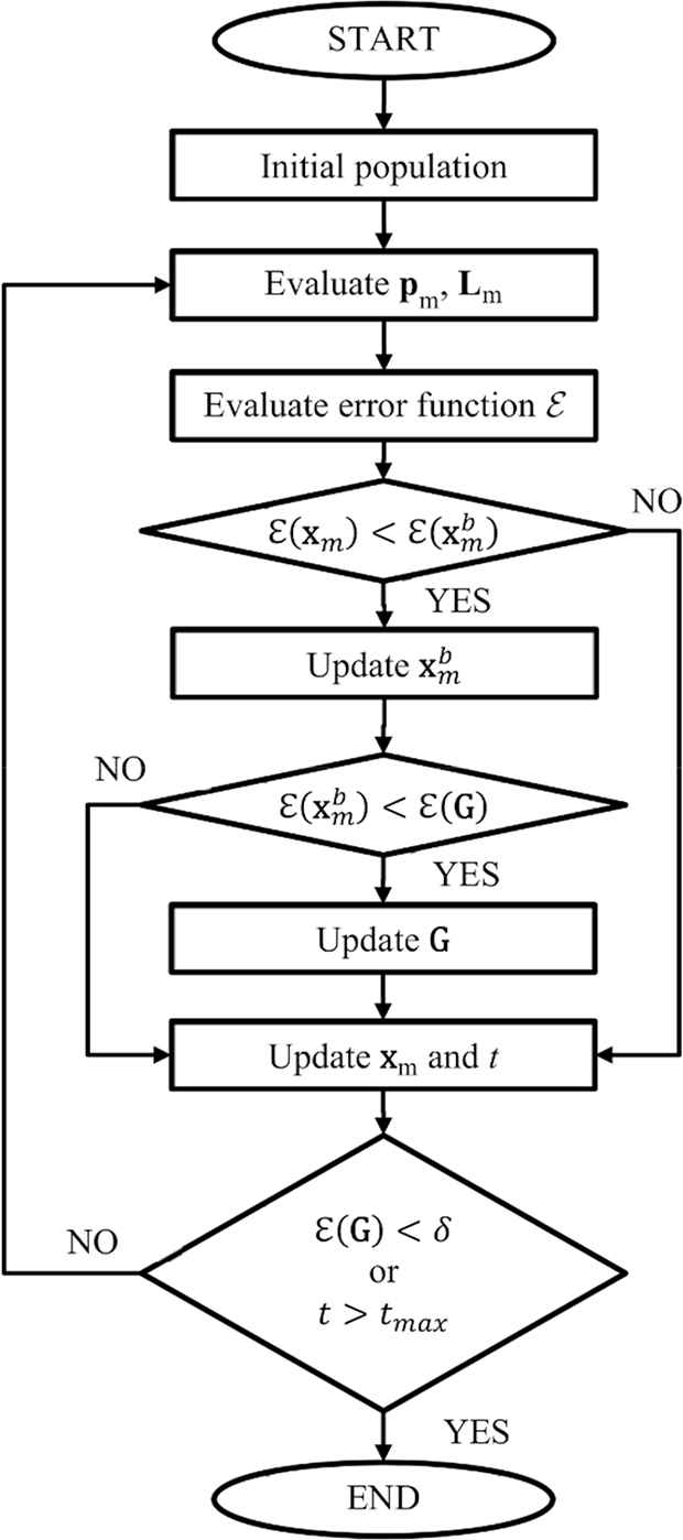
Flowchart of the EWQPSO algorithm regarding the minimization problem.
4. BENCHMARK TESTS FOR THE EWQPSO ALGORITHM
Several tests have been carried out to verify the effectiveness and performance of the proposed EWQPSO algorithm. In particular, the minimum searching problems regarding the Alpine and De Jong test functions are considered by changing both the domain dimension N and the number of particles M [8,23]. The maximum generation value is set to tmax = 500 + 10N. For each function, the results calculated by using EWQPSO, WQPSO, and QPSO algorithms have been compared. The search algorithm is applied 100 times for each test function, and the mean and standard deviation values relevant to the best particle have been calculated.
4.1. Alpine Test Function
The Alpine function is defined as follows:
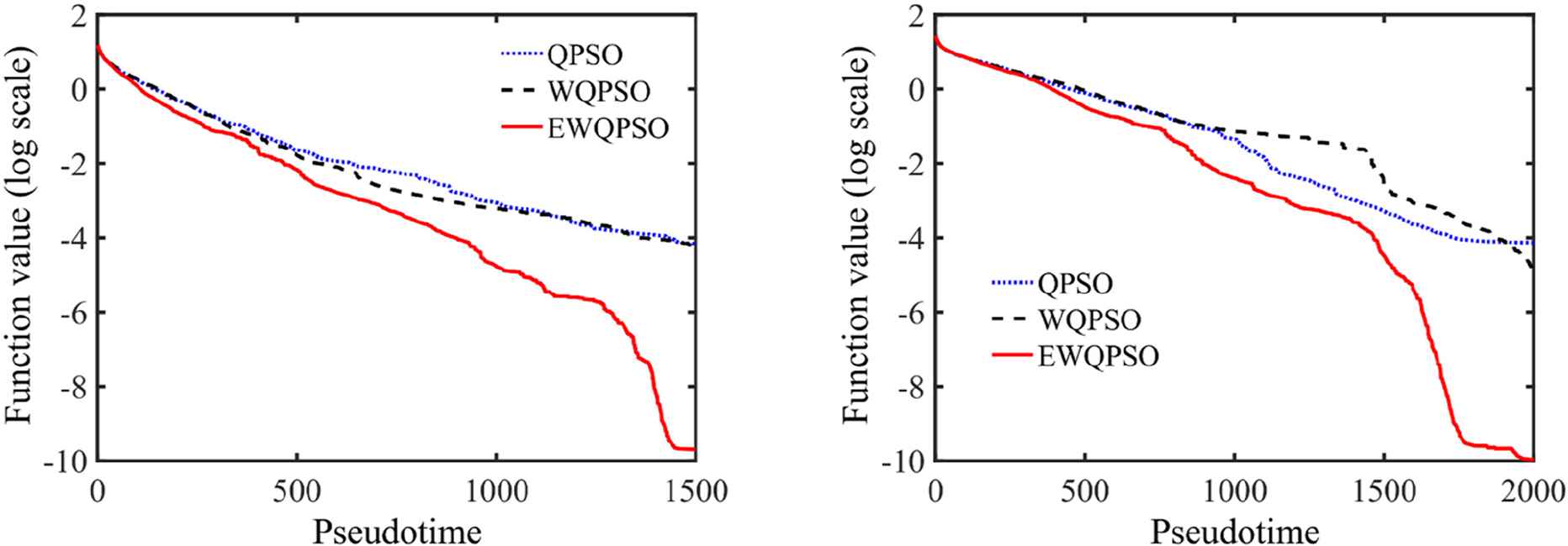
Evolution of the mean value corresponding to the best particle position of the EWQPSO, WQPSO and QPSO applied to the Alpine function for N=10 (left) and N=15 (right). A swarm composed of M = 30 particles is considered.
4.2. De Jong Test Function
The de Jong function is defined as follows:
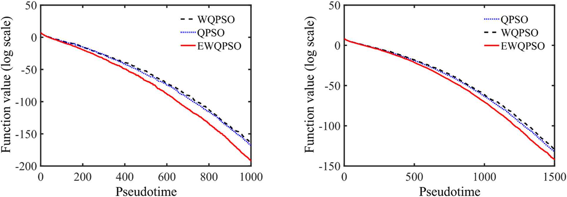
Evolution of the mean value corresponding to the best particle position of the EWQPSO, WQPSO and QPSO applied to the de Jong function for N=5 (left) and N=10 (right). A swarm composed of M = 30 particles is considered.
In Table 1 are listed the mean and standard deviation (STD) values taking into account the minimum value associated with the best particle found in each of the 100 runs and by changing the particle number and the test function. By visual inspection of the results, one can easily conclude that the developed EWQPSO algorithm is characterized by improved accuracy.
| Test Function | N | QPSO | WQPSO | EWQPSO | |||
|---|---|---|---|---|---|---|---|
| Mean | STD | Mean | STD | Mean | STD | ||
| Alpine | 5 | 3.63e-5 | 1.64e-4 | 7.99e-5 | 4.70e-4 | 1.42e-6 | 8.31e-6 |
| 10 | 6.94e-5 | 3.10e-4 | 6.35e-5 | 3.61e-4 | 2.05e-10 | 1.74e-9 | |
| 15 | 7.46e-5 | 7.45e-4 | 9.23e-6 | 6.11e-5 | 1.08e-10 | 1.08e-9 | |
| 20 | 5.50e-4 | 5.50e-3 | 5.09e-4 | 3.63e-3 | 2.51e-4 | 1.77e-3 | |
| de Jong | 5 | 1.27e-169 | 6.48e-169 | 9.32e-165 | 6.56e-164 | 6.37e-193 | 6.05e-192 |
| 10 | 3.58e-133 | 2.73e-132 | 1.00e-130 | 9.31e-130 | 1.04e-142 | 1.00e-141 | |
| 15 | 3.31e-104 | 1.44e-103 | 1.50e-101 | 7.46e-101 | 2.35e-108 | 1.92e-107 | |
| 20 | 3.72e-81 | 2.59e-80 | 3.40e-80 | 1.80e-79 | 2.29e-84 | 1.34e-83 | |
Mean and STD values of the global best particle calculated using the EWQPSO, WQPSO and QPSO algorithms and considering different test functions.
5. EWQPSO FOR SUPERSHAPED LENS ANTENNA SYNTHESIS
Researchers and engineers have shown extensive interest in dielectric lens antennas due to their potential use in various fields, such as wireless communication systems, smart antennas and radar systems. These antennas are attractive because they are easy to integrate and have the ability of shaping and collimating beams. In the past, most research was focused on developing 3D dielectric lenses with simple geometries, but recent studies have explored complex shapes using Gielis’ superformula [27,28,29,30]. This formula allows for generating a wide range of 3D shapes by changing a few parameters, which can be optimized using an automated procedure based on the QPSO algorithm.
The surface of the lens can be described by the following Gielis’ equations in a Cartesian coordinate system:
Fig. 4 shows the antenna structure used in the synthesis procedure. It consists of a large dielectric lens placed in the center of a circular plate made of electrically conductive material. The plate acts as a ground plane and also helps to reduce back-scattered radiation. The lens is illuminated by the electromagnetic field emitted by an open-ended circular waveguide filled with the same dielectric material as the lens. The propagation of the electromagnetic waves inside the lens is modeled using the tube tracing approach based on the combined geometrical optics/physical optics (GO/PO) approximation. This approximation allows significant simplification of the mathematical model making the simulation of electrically large structures possible with a lower computational effort than full-wave numerical methods. In fact, by virtue of the GO/PO approximation, the traveling electromagnetic wave can be approximated by a set of tubes propagating over a rectilinear path inside the lens [31,32,33]. The accuracy of the method can be further improved by considering the effects of multiple internal reflections occurring within the lens.
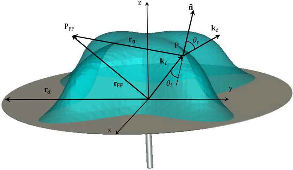
Structure of a supershaped dielectric lens antenna.
The developed GO/PO tube-tracing algorithm has been validated by comparison with the full-wave finite integration technique (FIT) adopted in the commercially available electromagnetic solver CST Microwave Studio [31,32,33]. A dedicated novel synthesis procedure based on EWQPSO is adopted to design a particular lens antenna showing a fixed 3D radiation pattern at frequency f=60 GHz. Such antennas could improve the channel capacity in communication systems implementing spatial-division multiplexing. The lens is made from a dielectric material with relative permittivity equal to εr= 2, the cylindrical open-ended waveguide and the metal plate have diameter dw = 2.3 mm and d = 20 cm, respectively. A swarm of M=48 particles has been launched over a maximum pseudo-time tmax = 40. The position vector relevant to the m-th particle is
The developed modeling technique is adopted to synthesize a lens antenna featuring a radiation beam pattern with four main lobes at the frequency f=60 GHz. This type of antenna could be adopted in communication systems implementing a spatial division multiplexing useful for increasing the channel capacity where the position of the receiver is known. The fitness function value is evaluated as:
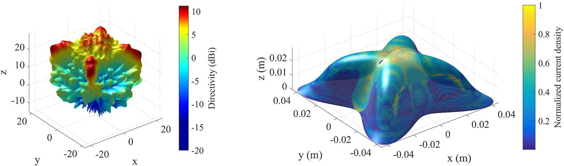
Radiation solid (left) generated by the current density distribution (right) on the lens surface.
Fig. 6 shows both the target and EWQPSO recovered polar section of the radiation solids. It is worth noting that the synthesized radiation patterns are in excellent agreement with the target masks. Moreover, it is apparent that accounting for the multiple wave reflections occurring within the lens is instrumental to the enhancement of the modeling accuracy of the procedure. Fig. 7 shows the convergence rate of the new optimization procedure (EWQPSO) when applied to the synthesis of the lens antenna illustrated in Fig. 5. The convergence of the average value of the fitness function of the whole swarm to the one corresponding to the global best demonstrates the capability of the entire swarm to search the optimal solution effectively.
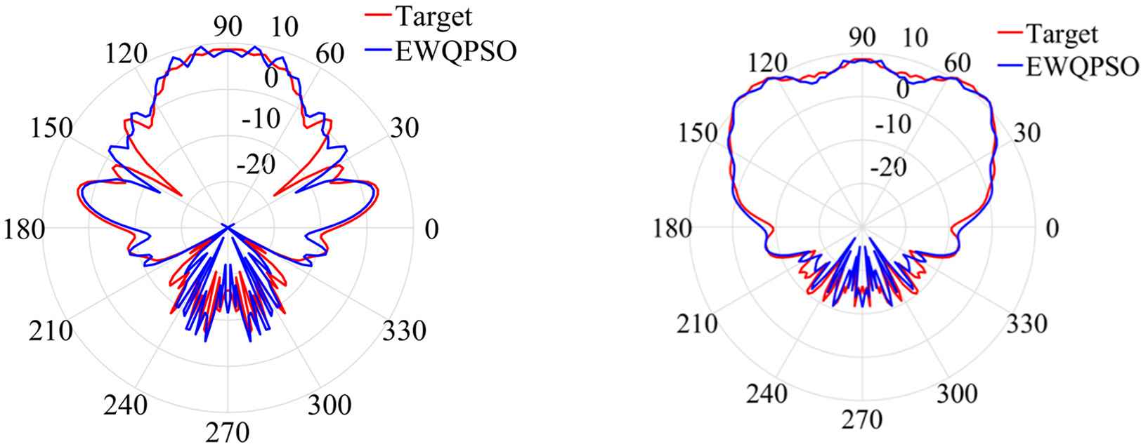
Comparison between the target directivity and the directivity of the Gielis’ lens antenna synthesized by means of the EWQPSO procedure: ϕ = 0° (left) and ϕ = 45° (right).
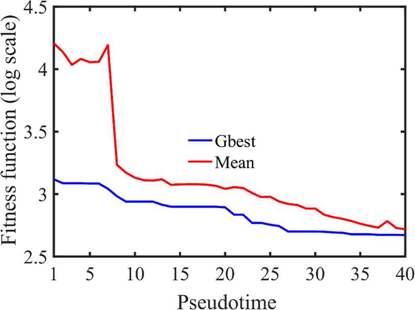
Convergence rate of the EWQPSO procedure.
The lens antenna structures shown in the illustrations have specific radiation pattern properties that can be beneficial for the newly introduced Wi-Fi 802.11ad communication protocol at a frequency of 60 GHz. Previously published articles by the authors [20,34] have demonstrated the effectiveness of the proposed EWQPSO model in designing a particular class of dielectric lens antennas defined by the Gielis formula. The EWQPSO technique outperforms classical PSO and genetic algorithms (GAs), as well as the conventional WQPSO procedure, in terms of convergence rate, accuracy and population size. These properties are desirable in the considered context as the computational burden associated with the computation of the fitness function is significant.
6. CONCLUSION
This research study has illustrated an optimization algorithm, EWQPSO, based on the quantum-behaved PSO approach, to solve complex electromagnetic problems. Comparative analysis with conventional QPSO and WQPSO algorithms indicates that EWQPSO is faster and more accurate.
The EWQPSO algorithm is applied to the solution of inverse problems concerning the determination of the Gielis parameters of supershaped dielectric lens antennas with multi-beam characteristics at mm-wave frequencies. The obtained results demonstrate the effectiveness of the proposed approach in identifying optimal solutions. Additionally, the algorithm is easy to implement, as it does not require the evaluation of complicated evolutionary operators or a large number of synthesis parameters. Even when using the generalized Gielis formula [35], with additional design parameters, the same algorithm can be applied [36]. This makes it an appealing and efficient alternative tool for designing and characterizing these types of antennas.
REFERENCES
Cite This Article
TY  - CONF
AU  - Luciano Mescia
AU  - Pietro Bia
AU  - Johan Gielis
AU  - Diego Caratelli
PY  - 2023
DA  - 2023/11/29
TI  - Advanced Particle Swarm Optimization Methods for Electromagnetics
BT  - Proceedings of the 1st International Symposium on Square Bamboos and the Geometree (ISSBG 2022)
PB  - Athena Publishing
SP  - 109
EP  - 122
SN  - 2949-9429
UR  - https://doi.org/10.55060/s.atmps.231115.010
DO  - https://doi.org/10.55060/s.atmps.231115.010
ID  - Mescia2023
ER  -


