Proceedings of the 1st International Symposium on Square Bamboos and the Geometree (ISSBG 2022)

Umbral Calculus and New Trigonometries
Downloads:
311
Full-Text Views:
75
Citations (Scopus):
0
Citations (Crossref):
0
Cite This Article

1. INTRODUCTION

The term Umbra1 has been diffused by S. Roman and G.C. Rota [1] in the second half of the 20th century to underline, in the emerging field of operational calculus, the practice of replacing the representation in series of certain function fx with the formal exponential series2. Earlier, other mathematicians like J. Blissard in Theory of Generic Equations or Edouard Lucas in Théorie nouvelle des nombres de Bernoulli et d'Euler, established the rules which allowed for viewing different functions through the same abstract entity and showed its usefulness for a wide range of applications. In the current research, the same starting point has been used but with methods closer to the Heaviside point of view [2], by proposing strategies combining different technicalities and operational methods which yield the formulation of a powerful “different mathematical language” [3]. The umbral image, the key element to establish the rules to replace higher transcendental functions in terms of elementary functions, and rewrite complex problems into simplified exercises, will be the starting point to fix the criteria to take advantage from such a replacement, based on the Laplace and Borel transform Theory and the Principle of Permanence of the Formal Properties.

To introduce the umbral operator, we have to provide some preliminary definitions. The operator c^, called umbral, is a shift operator c^=ez acting on an appropriate chosen vacuum3, which is a function that will change according to the problem to solve [3]. If the initial vacuum is, for example, the function:

φμ:=φμ= 1Γμ+1          μ(1)
the umbral operator c^ μ, μ, will be the action of the operator c^ on the vacuum φ0 such that:4
c^ μφ0:=φμ=1 Γμ+1(2)

By that definition, the operator c^ has the properties of the standard exponential c^ ±μc^ ν=c^ ±μ+ν and  c^ ±μν=c^ ±μ ν,μ,ν. In the following we list a plethora of examples of applications of the umbral operator. We start with the creation of the umbral image of some special function.

2. SPECIAL FUNCTIONS

By using the operator in Eq. 25 and the property of Γ-functions [4], we find the umbral image of the Bessel function [5]. Indeed, by exploiting the series representation of the Bessel function, we get, x:

J0x=r=01rx22rr!2=r=0d1rx22rc^ rr!φ0=ec^x22φ0(3)
obtaining in this way a new formulation of Bessel function in terms of the Gaussian function. We can furthermore write the umbral n-order Bessel function:
Jnx=r=01rx22r+nr!r+n!=c^x2ec^x22φ0          x(4)

So we have formally reduced a transcendental function to an exponential form, downgrading the “complexity” of the function.

The umbral image is not unique indeed, if we chose another vacuum, the action of the umbral operator will yield a different function. For example, if we introduce the pair umbral operator/vacuum such that:

b^ rΦ0:=Φr=1Γr+12          r(5)
we obtain:
J0x=r=01rr!2x22r=r=01rx22rb^ rΦ0=11+b^x22Φ0          x(6)
thus expressing the Bessel function in a rational form, according to operator b^ and the vacuum Φ0. Obviously, the umbral images are “equivalent” in the sense that the mathematical problems including the initial function (in the present example, the Bessel function) can be treated indifferently through the first of the second proposed umbral image, as shown below.

Example 1.

x

J0xdx =ecˆx22dxφ0=2πcˆφ0=2πcˆ12φ0=2π1Γ12+1=2(7)
J0xdx =11+bˆx22dxΦ0=2πbˆΦ0=2πbˆ12Φ0= 2πΓ122=2(8)

This kind of new “interpretation” of a certain function opens a wide range of possibilities. To this aim, we provide some examples including the solution of non-trivial integrals.

Example 2.

We consider integrals involving the Bessel function J0 and the umbral operator c^ [3,6]. Then a,b:ax2+bx>0:

IJa,b= J02ax2+bxdx=ecˆax2+bxdxφ0=πcˆaecˆb24aφ0=πab2aI 12ba (9)
where Iνx is a modified Bessel function of the first kind, or a,b+:
IL,Ja,b=J02ax1+bx21+bx2dx=πbr=0Γr+12r!3abr(10)

Furthermore, we want to stress the possibility to evaluate the product of special functions by using the umbral images. However, we recall that in general the operator is not commutative. So if we want to calculate, for example, J0x2 we cannot use the same operator raised to power 2, but we have to define two different operators acting on two different vacua in the following way. We get a,b,x [7]:

J0ax=ea2cˆ1x22φ0,1           J0bx=eb2cˆ2x22φ0,2(11)
and introduce the function fx;a,b:=J0axJ0bx. Then [7]:
fx;a,b=ea2cˆ1+b2cˆ2x22φ0,1φ0,2(12)

By expanding the exponential in MacLaurin series we can finally write:

fx,a, b=r=0(1)rr!lra2, b2χ22rlra, b=r!s=0rarsbs(s!)2[rs!]2(13)
hence finding a closed formula for a non-trivial product of special functions.

2.1. Hermite Polynomials

We consider now the two-variable polynomials of Hermite Kampé dè Fériét [4,8,9], also called heat polynomials:

Hnx,y=n!s=0n2xn2sysn2s!s!         x,y, n(14)
with generating function [3]:
r=0tnn!Hnx,y=ext+yt2(15)

From an operational point of view, they can be expressed as the result of the action of the operator x2 on the monomial xn:Hnx,y=eyx2xn [5,10]. In a geometrical sense we understand the operational rule as the transformation of the exponential operator on an ordinary monomial into a Hermite type special polynomial. The “evolution” from an ordinary monomial to the corresponding Hermite is shown by moving the cutting plane orthogonal to the y axis (Fig. 1). For a specific value of the polynomial degree n, the polynomials lie on the cutting plane. For negative values of y they realize an orthogonal set [3,11]. By using the umbral technique [1], we can extend the Hermite polynomial representation to Hermite function representation [10,11], considering the order ν and exploiting the Newton binomial and the Laplace transform [4,12,13,14], as shown below.

Figure 1

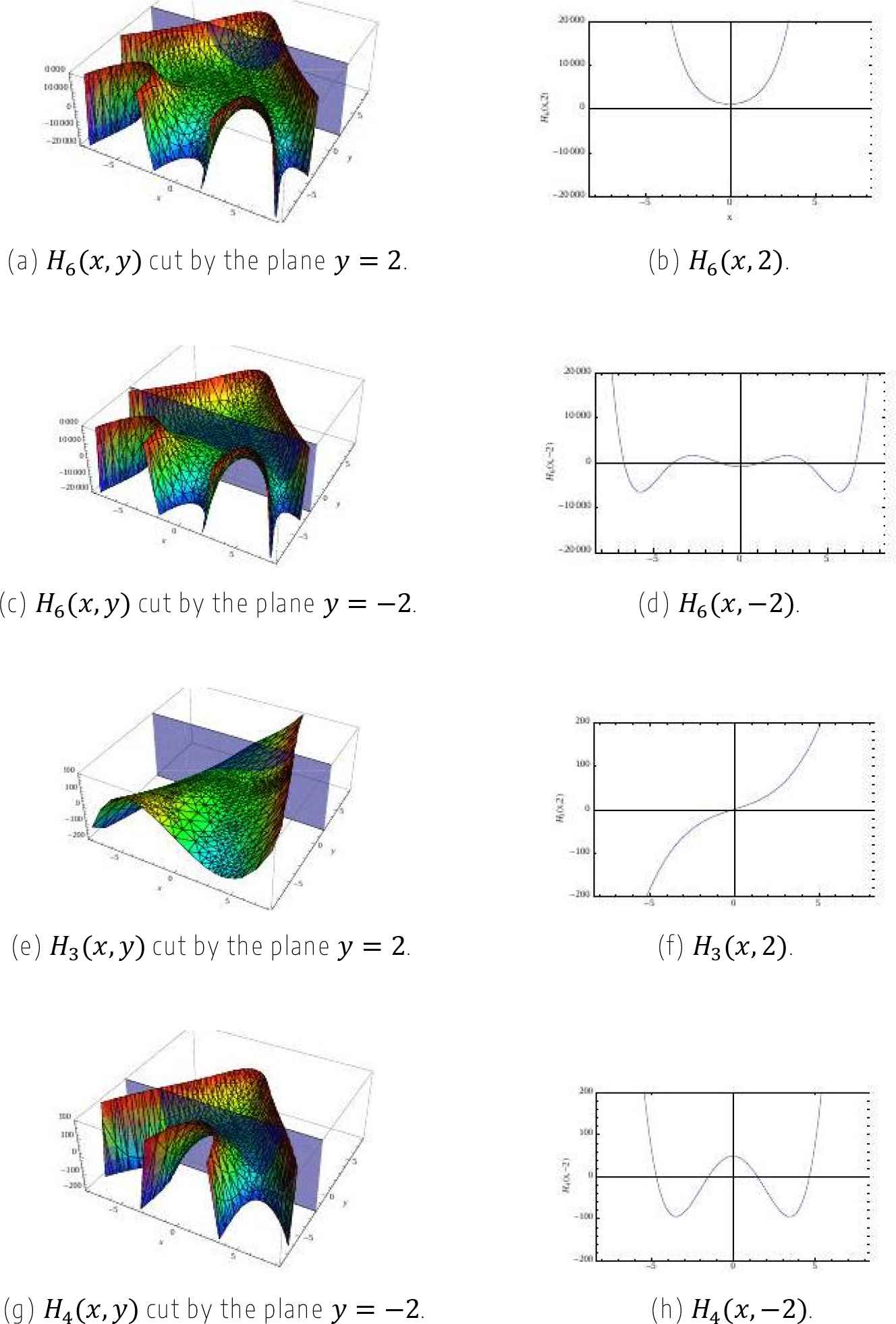
Geometrical representation of two-variable Hermite polynomials in 3D and 2D for different n and y values.

Proposition 1.

Hnx,y=x+ yhˆnθ0         x,y,n(16)
with  yhˆ umbral operator and θ0 vacuum such that:
 yhˆrθ0:=θr=yr2r!Γr2+1cosrπ2=0   r=2s+1ys2s!s!   r=2s     s(17)

Proof.

By considering the definition of the  yhˆ operator we can write:

x+ yhˆnθ0 =r=0nnrxnr yhˆrθ0=r=0nnrxnrys2s!s!=s=0n2xn2sysn!n2s!s!=Hnx,y(18)

Proposition 2.

The relevant Hermite function integral representation, with order real and negative too, can be written as:

Hνx,y=1Γν0sν1esxeys2ds          x,y,ν+(19)

Proof.

By considering the definition of the  yhˆ operator we can write:

Hνx,y=1x+ yhˆνθ0=0exssν1eyhˆsΓνdsθ0=1Γν0sν1esxeys2ds

Furthermore, if we introduce another application of the umbral methods, called Hermite calculus [15], we can reach the target to combine the previous results and calculate, for example, non-trivial integrals including combination of special functions. To give an idea of the methods we will use, we consider the following integral:

Iα,β,γ=eα+βx2γxdx(20)
which can be evaluated through the Gauss-Weierstrass integral [3]:
Iα,β,γ=πα+βeγ24α+β(21)
but we recast the integral in Eq. (20) in umbral form:
Iα,β,γ=eαx2hˆγ,βxdx(22)
where we introduced the umbral operator hˆ.,. and the vacuum η0 such that:
hˆx,yrη0:=Hrx,y(23)

By that position, we can recast:

ehˆγ,βx=r=0(x)rr!hˆγ,βr=r=0(x)rr!Hrγ,β(24)
and by treating the umbral operator hˆ.,. as an ordinary algebraic quantity, as explained previously, we can solve the integral in Eq. (22) in the form:
Iα,β,γ=παehˆγ,β24αη0=παr=01r!hˆγ,β24αrη0=παr=01r!H2rγ2α,β4α=πα+βeγ24α+β(25)

In this way, we have shown the flexibility of the technique. Indeed, we can raise the complexity of the integrals and solve them by methods as, for example, in the case of the anharmonic oscillator in the example below [15,16].

Example 3.

Let:

Ja,b,c=eax4+bx2+cxdx         Rea>0(26)

be the integral of the anharmonic oscillator. We can solve it by the Hermite calculus position:

Ja,b,c=ehˆb,ax2cxdx=πhˆec24hˆ=πs=01s!c22shˆs+12(27)

in which we used the fractional order of the umbral operator and of the Hermite function:

hˆs+12=Hs+12b,a(28)

The same consideration can be done for each special function through appropriate umbral images. We list in the following just some examples for the Laguerre, Jacobi, Legendre, Tricomi-Bessel and Chebyshev functions, and the Voigt transform [12,17,18].

LaguerreLnx, γ=(γc^x)nϕ0JacobiPnα,βz=Γn+α+1Γn+β+1n!2Rnα,βx12,x+12Rnα,βξ, η=n!c^1αc^2β[c^1ξ+c^2η]nϕ1,0ϕ2ε0LegendrePnx=Rn0,0ξ,ηTricomi-BesselCvx=1χv2Jv2χChebyshevUnx, y=1n!0esxs+(ys)h^nθ0dsVoigtvf^x,y;z=0extyt2fztdt
and so on.

3. NUMBER THEORY

The umbral method can be applied in many different fields of pure and applied mathematics. A further example is indeed Number Theory. We remind that Harmonic Numbers are defined as [19,20,21,22]:

hn:=r=1n1r          n0(29)

In terms of Laplace transform, we obtain:

hn=r=1n0esrds          n0(30)
thereby getting the n-th harmonic number through Euler's integral:
hn=011xn1xdx(31)
valid more generally n+.

We can then introduce the function:

φhz:=φhz=011xz1xdx          z+(32)
as the Harmonic Number Umbral Vacuum:
h^ nφh0=h^ nφhzz=0 =enzφhzz=0=φhz+nz=0=011xz+n1xdxz=0=011xn1xdx=hn(33)
and, without dwelling on the details5, introduce the Harmonic Based Exponential Function as the series:
 hex:=ehˆx=1+n=1hnn!xn          x (34)

In an analogous way, we can treat other families of numbers like the Motzkin, telegraph, Stirling numbers, etc.

4. CLASSIC TRIGONOMETRY

Trigonometry can also be reinterpreted in terms of umbral images.

Definition 1.

We introduce, α,β+, the umbral vacuum:

ψκ:=Γκ+1Γακ+β          κ(35)
and the shift operator  α,βdˆ such that we can get:
 α,βdˆκψ0=Γκ+1Γακ+β(36)

Proposition 3.

(Cos-exponential umbral image) If α=2 and β=1,x:

cosx=r=0(1)rx2r2r!=r=0(1)rx2rr! 2,1dˆrψ0=e2,1dˆx2 ψ0(37)
as we expect.

Corollary 1.

x:

xe2,1dˆx2ψ0=2x  2,1dˆe 2,1dˆx2ψ0=2xr=0(1)rr+1!2r+2!x2rr!=r=0(1)rx2r+12r+1!=sinx(38)

Fresnel Integral [17]:

Cx=x+cosξ2dξ          x(39)
C0=0+e2,1dˆx4ψ0dx=140eyy141dydˆ2,114ψ0= 14Γ14Γ34Γ12= 12π2(40)

By applying the methods discussed so far, we can put together integrals including trigonometric functions and Hermite polynomials [23] and solve them in a simple way.

Example 4.

axHnξ,y cos ξdξ=s=0n cos x+s+1π2n!ns!Hnsx,y+n! cos n+1π21n12en12yemx=r=0mxrr!truncatedexponentialfunctionayHnx,η cos ηdη=s=0n2 cos y+s+1π2n!n2s!Hn2sx,y+n!(1)n244en2(1)14x[k]em(x)=r=0mkxmkrmkr!truncatedexponentialfunctionoforderk(41)

5. NEW TRIGONOMETRIES AND THE GIELIS SUPERFORMULA

We wish to close this contribution with a view on new trigonometries and the Gielis Superformula.

Definition 2.

We introduce the composition rule x,y,n:

 leylxxn=r=0nnr2xnryr:=xlyn(42)
called the Laguerre binomial sum.

Eq. (42) is based on the Laguerre exponential [24,25]:

 leη:=r=0ηrr!2          η(43)
in which the argument of the function includes the Laguerre derivative  lx and the binomial coefficient has exponent 2 instead of 1 in the ordinary Newton binomial. Then, in full analogy with the ordinary Euler formulae, we introduce the following:

Definition 3.

We introduce l-trigonometric (l-t) functions through the identity:

 leix= lcx+iιsx(44)
where l − t cosine and l − t sine functions are specified by the series6 (Fig. 2):
 lcx=r=0(1)rx2r2r!2 ,         lsx=r=0(1)rx2r+12r+1!2(45)

We can also use matrices as arguments of the l-sin or l-cos functions (like in PDE system problems): see Fig. 3.

Figure 2

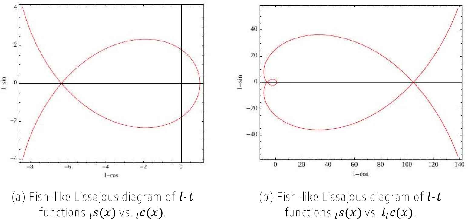
Examples of l-trigonometric functions.

Figure 3

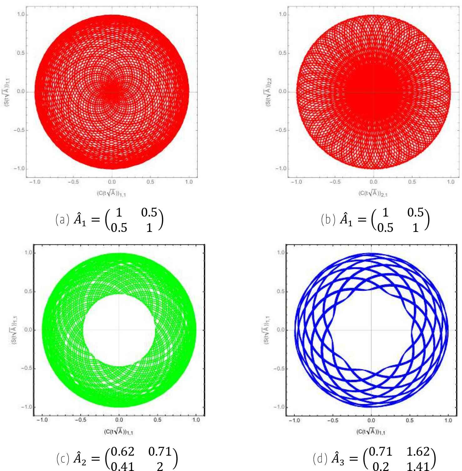
Examples of l-trigonometric functions with matrices as arguments: S(tAˆ) vs. C(tAˆ).

Finally, by using the Superformula of Johan Gielis [26], a wide range of novel shapes can be generated (Fig. 4). n1,n2,n3,m,a,b+,a,b0,θ,r=rθ radius:

1r=1acosm4θn21bsinm4θn3n1(46)

Figure 4

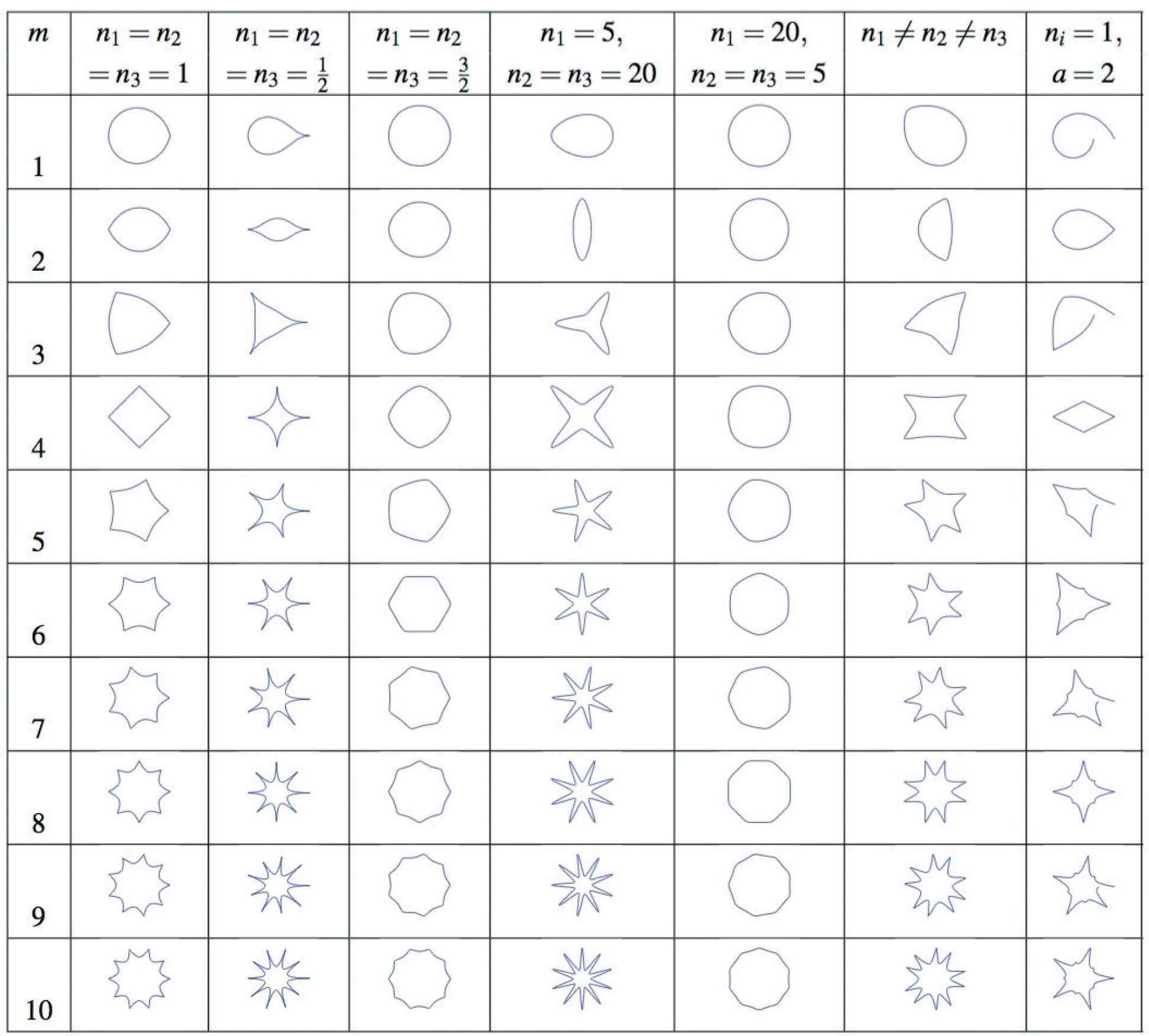
Table of various shapes.

We can identify cos lcos and sin lsin and repeat the procedure as in the previous sections, so yielding “strange” and lovely new figures in 2D and 3D (Fig. 5).

Figure 5

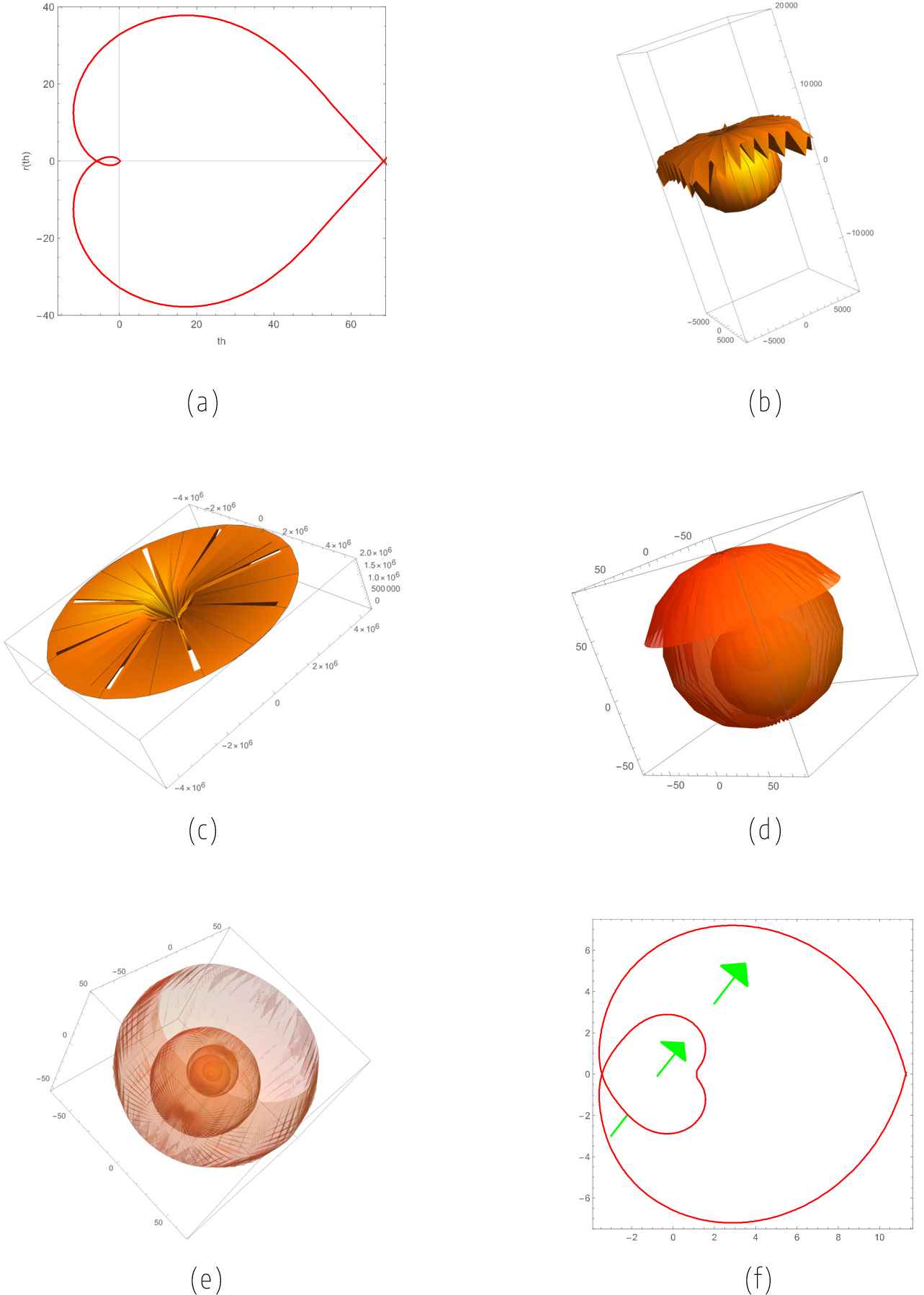
(a) Heart. (b) Strange fruit. (c) Strange leaf. (d) Nut. (e) Tulip. (f) Loving hearts.

ACKNOWLEDGMENTS

This work was supported by an ENEA Research Center individual fellowship and under the auspices of INDAM's GNFM (Italy).

Footnotes

It is assonant to the term “Ombra” in Latin which means “shadow” in English.

The promotion of the index n in cn to a power exponent of the operator ĉ, the umbral operator, is the essence of umbra, since it is a kind of projection of one into the other: fx=n=0cnxnn! n=0c^xnn!=ec^x

This term is used to stress that the action of the operators, raised to some power, is that of acting on an appropriate set of functions by “filling” the initial state φ0= 1 Γ1 (see [3] for a rigorous treatment of the topic).

c^ μφ0=eμzφzz=0=φz+μz=0= 1 Γz+μ+1z=0= 1 Γμ+1

See [20] for more details.

The l-t functions are defined by the corresponding series expansion lchx=r=0x2r[2r!]2, lshx=r=0x2r+1[2r+1!]2

REFERENCES

S.M. Roman, G.-C. Rota. The Umbral Calculus. Advances in Mathematics, 1978, 27(2): 95–188. https://doi.org/10.1016/0001-8708(78)90087-7
P.J. Nahin. Oliver Heaviside: The Life, Work, and Times of an Electrical Genius of the Victorian Age. Baltimore: Johns Hopkins University Press, 2002.
S. Licciardi, G. Dattoli. Guide to the Umbral Calculus: A Different Mathematical Language. Singapore: World Scientific, 2022. https://doi.org/10.1142/12804
M. Abramowitz, I.A. Stegun. Handbook of Mathematical Functions: With Formulas, Graphs, and Mathematical Tables, 9th revised edition. New York: Dover Publications, 1972.
D. Babusci, G. Dattoli, S. Licciardi, E. Sabia. Mathematical Methods for Physicists. Singapore: World Scientific, 2019. https://doi.org/10.1142/11315
G. Dattoli, B. Germano, S. Licciardi, M.R. Martinelli. Integrals of Special Functions and Umbral Methods. International Journal of Applied and Computational Mathematics, 2021, 7(4): 120. https://doi.org/10.1007/s40819-021-01047-w
G. Dattoli, E. Di Palma, E. Sabia, S. Licciardi. Products of Bessel Functions and Associated Polynomials. Applied Mathematics and Computation, 2015, 266: 507–514. https://doi.org/10.1016/j.amc.2015.05.085
P. Appell, J. Kampé de Fériet. Fonctions Hypergeìomeìtriques et Hyperspheìriques: Polynomes d'Hermite. Paris: Gauthier-Villars, 1926. (in French)
G. Dattoli, B. Germano, P.E. Ricci. Hermite Polynomials With More Than Two Variables and Associated Bi-Orthogonal Functions. Integral Transforms and Special Functions, 2009, 20(1): 17–22. https://doi.org/10.1080/10652460801933678
G. Dattoli, B. Germano, P.E. Ricci. Comments on Monomiality, Ordinary Polynomials and Associated Bi-Orthogonal Functions. Applied Mathematics and Computation, 2004, 154(1): 219–227. https://doi.org/10.1016/S0096-3003(03)00705-7
M. Artioli, G. Dattoli. Geometry of Two-Variable Legendre Polynomials. Wolfram Demonstrations Project, 25 January 2016. http://demonstrations.wolfram.com/GeometryOfTwoVariableLegendrePolynomials/
G. Dattoli, B. Germano, S. Licciardi, M.R. Martinelli. On an Umbral Treatment of Gegenbauer, Legendre and Jacobi Polynomials. International Mathematical Forum, 2017, 12(11): 531–551. https://doi.org/10.12988/imf.2017.6789
L.C. Andrews. Special Functions for Engineers and Applied Mathematicians. New York: Macmillan, 1985.
J. Mikusiński. On the Function Whose Laplace-Transform is exp(−sa). Studia Mathematica, 1959, 18(2): 191–198. https://doi.org/10.4064/sm-18-2-191-198
G. Dattoli, B. Germano, S. Licciardi, M.R. Martinelli. Hermite Calculus. In: J. Gielis, P.E. Ricci, I. Tavkhelidze (Eds.), Modeling in Mathematics: Proceedings of the Second Tbilisi-Salerno Workshop on Modeling in Mathematics. Atlantis Transactions in Geometry, Vol. 2, pp. 43–52. Paris: Atlantis Press, 2017. https://doi.org/10.2991/978-94-6239-261-8_4
J. Boháčik, P. August쬬 P. Prešnajder. Non-Perturbative Anharmonic Correction to Mehler's Presentation of the Harmonic Oscillator Propagator. Ukrainian Journal of Physics, 2014, 59(2): 179–192. https://doi.org/10.15407/ujpe59.02.0179
S. Licciardi, R.M. Pidatella, M. Artioli, G. Dattoli. Voigt Transform and Umbral Image. Mathematical and Computational Applications, 2020, 25(3): 49. https://doi.org/10.3390/mca25030049
N.M. Temme. Voigt Function. In: F.W.J. Olver, D.W. Lozier, R.F. Boisvert, C.W. Clark (Eds.), NIST Handbook of Mathematical Functions. Cambridge: Cambridge University Press, 2010.
J. Sondow, E.W. Weisstein. Harmonic Number. MathWorld – A Wolfram Web Resource. http://mathworld.wolfram.com/HarmonicNumber.html
G. Dattoli, H.M. Srivastava. A Note on Harmonic Numbers, Umbral Calculus and Generating Functions. Applied Mathematics Letters, 2008, 21(7): 686–693. https://doi.org/10.1016/j.aml.2007.07.021
R.W. Gosper. Harmonic Summation and Exponential GFS. Post on math-fun@cs.arizona.edu, 2 August 1996.
G. Dattoli, B. Germano, S. Licciardi, M.R. Martinelli. Umbral Methods and Harmonic Numbers. Axioms, 2018, 7(3): 62. https://doi.org/10.3390/axioms7030062
G. Dattoli, S. Licciardi. Operational, Umbral Methods, Borel Transform and Negative Derivative Operator Techniques. Integral Transforms and Special Functions, 2020, 31(3): 192–220. https://doi.org/10.1080/10652469.2019.1684487
G. Dattoli, E. Di Palma, S. Licciardi, E. Sabia. From Circular to Bessel Functions: A Transition Through the Umbral Method. Fractal and Fractional, 2017, 1(1): 9. https://doi.org/10.3390/fractalfract1010009
G. Dattoli, S. Licciardi, R.M. Pidatella. Theory of Generalized Trigonometric Functions: From Laguerre to Airy Forms. Journal of Mathematical Analysis and Applications, 2018, 468(1): 103–115. https://doi.org/10.1016/j.jmaa.2018.07.044
J. Gielis. A Generic Geometric Transformation That Unifies a Wide Range of Natural and Abstract Shapes. American Journal of Botany, 2003, 90(3): 333–338. https://doi.org/10.3732/ajb.90.3.333

Cite This Article

ris
TY  - CONF
AU  - Silvia Licciardi
PY  - 2023
DA  - 2023/11/29
TI  - Umbral Calculus and New Trigonometries
BT  - Proceedings of the 1st International Symposium on Square Bamboos and the Geometree (ISSBG 2022)
PB  - Athena Publishing
SP  - 95
EP  - 106
SN  - 2949-9429
UR  - https://doi.org/10.55060/s.atmps.231115.009
DO  - https://doi.org/10.55060/s.atmps.231115.009
ID  - Licciardi2023
ER  -
enw
bib