
Revised 10 June 2023
Accepted 9 October 2023
Available Online 29 November 2023
- DOI
- https://doi.org/10.55060/s.atmps.231115.008
- Keywords
- Mittag-Leffler polynomials
Umbral formalism(s)
Monomiality formalisms - Abstract
The theory of special polynomials, and of special functions as well, is greatly simplified by the use of algebraic methods of umbral nature. In this article we embed the umbral and monomiality formalism to study special polynomials expressed in terms of lower factorial polynomials. We touch on the theory of Mittag-Leffler polynomials and derive the relevant properties using elementary means. We also provide a general description of non-standard partial differential equations, playing a central role in the theory of this family of polynomials.
- Copyright
- © 2023 The Authors. Published by Athena International Publishing B.V.
- Open Access
- This is an open access article distributed under the CC BY-NC 4.0 license (https://creativecommons.org/licenses/by-nc/4.0/).
1. INTRODUCTION
Methods based on the formalisms of monomiality [1,2] and/or umbrality, in their different declinations [3,4,5,6,7,8,9,10], have been useful tools to simplify and unify the treatment of special functions and polynomials.
Within the first point of view, special polynomials are reduced to ordinary monomials, while the latter can be exploited to reduce higher transcendent to elementary functions. The Bessel functions can e. g. be viewed as ordinary Gaussians and the Hermite or Laguerre polynomials can be treated as ordinary Newton binomials [9,10].
In this article we apply the technicalities of the monomiality/umbral formalism to study polynomials belonging to families (like the Mittag-Leffler polynomials and the relevant generalizations [11,12]) which can be expressed as combinations of lower factorial polynomials (l.f.p.).
The interest in the problem is due to the possibility of combining different algebraic procedures, offering significant simplifications, for the derivation of the relevant properties.
The lower factorial polynomials are expressed in terms of the Pochhammer symbol [13] as:
They belong to the family of Sheffer sequences [14] and are monomials [1,2] under the action of the derivative
Within the context of monomiality the
The last of which, written in terms of the differential realization of the operators
Furthermore, the multiplicative operator allows to construct the associated QM polynomial according to the identity:
Where 1 is the monomiality vacuum (see final comments in Section 4). Regarding the case under study, we find:
The generating functions of any quasi-monomial can therefore be cast in the form:
Regarding the lower factorial polynomials we obtain:
The last identity deserves further comments, useful for next developments.
According to the previous remarks, it is evident that:
Namely,
The concept and the technicalities that we have outlined in these introductory notes will be exploited in the forthcoming sections to develop a self-consistent theory of l.f.p. based polynomials.
2. EMBEDDING UMBRAL AND MONOMIALITY FORMALISMS
The umbral formalism (as conceived in [9,10] and references therein) is a fairly natural extension of the monomiality point of view. The generating function of l.f.p. in terms of umbral operators can be written as:
If
The notion of vacuum, albeit discussed in the quoted references concerning the umbral calculus, will be touched on in the concluding comments.
We can now combine the umbral and monomiality formalism, by noting that:
Accordingly, the exponential umbral function in Eq. (10) satisfies the identity:
Furthermore, the cos-like expansion:
In terms of ordinary variables, we evidently obtain that:
As a further example, aimed at completing the scenario of how to embed the prescribed algebraic tools, we underscore that it is possible to construct new and meaningful families of polynomials.
We consider therefore a polynomial defined in terms of the Newton binomial:
The polynomials
It is interesting to note that the generating function of the polynomials in Eq. (20) writes:
The key point is now that of specifying the mathematical meaning of
The function in the second equation of Eq. (22) is the umbral version of the zero-th order Tricomi-Bessel function [9,10].
The ordinary Tricomi-Bessel function is an eigenvalue of the Laguerre derivative [1,2], namely:
We find therefore that its umbral extension is an eigenvalue of:
Therefore we find:
The above eigenvalue problem reduces to a difference equation, which will be discussed elsewhere.
The polynomials in Eq. (20) can be interpreted as an umbral image of the Laguerre polynomials. They can indeed be written as:
Remaining within the same context we like to stress that Hermite-like polynomials can be constructed using an operational relationship, which, adapted to the case under study, reads (for the introduction of two-variable Hermite polynomials, see [15]):
These last identities can also be viewed as a particular solution of a generalization of the heat equation, commented in Section 4, along with other relevant technicalities of the formalism we are developing.
3. MITTAG-LEFFLER POLYNOMIALS
In Section 2 we introduced Laguerre-like polynomials, using a composed umbral procedure. Let us now take advantage from the formalism to note that, by keeping the derivative of both sides of Eq. (27) with respect to the variable
A family of polynomials associated with the generalized Laguerre [16] has been introduced in the past [17] as:
We get therefore:
Finally, multiplying the right side of Eq. (31) by
The Mittag-Leffler polynomials are well documented in mathematical literature since their introduction in 1891 (see [11,12]) and are defined as:
It is therefore evident (see Eq. (32) and Eq. (33)) that we can establish the following identity:
According to the previous identity, the Mittag-Leffler polynomials can be viewed as an umbral extension of the Laguerre family.
It is furthermore interesting (and straightforward) to obtain the generating function:
In a forthcoming dedicated investigation, we will see how old and new results on Mittag-Leffler polynomials and generalizations can be obtained within the framework of the formalism we have illustrated so far.
4. FINAL COMMENTS
In the course of the previous sections, we have described the details of an operational formalism, but we have left poorly justified some points.
The concept of vacua regarding monomials and umbral techniques, albeit justified in the dedicated literature, is worth to be underscored here.
4.1. Monomials
We consider the specific example of Hermite polynomials, whose multiplicative operator is realized as:
If it is raised to any integer, the Burchnall rule [18,19] yields the following identity:
It is evident that, if acting on a constant, for simplicity 1, it yields:
If not, namely if the multiplicative operator is applied to any function
If furthermore the function can be expanded in Hermite polynomials, namely:
The validity of identities of the type in Eq. (39) holds even for non-integer value of the exponent. Keeping
The last integral in Eq. (42) converges for
The formalism of quasi monomiality can be extended to non-integer “pseudo-Hermite” polynomials and it is easily checked that they satisfy the same recurrences of the ordinary Hermite [16]. This statement holds true for all the polynomial families defined as quasi monomials. But this suggestion will not be pursued in this article.
4.2. Umbral
The definition of umbral operator and of the associated vacuum has been discussed in sufficient detail in previous articles, for a more pedagogic discussion we address the reader to [9,10]. In the case of the l.f.p. they can be identified with:
Another point deserving clarification is the statement about the possibility of writing quasi monomial/umbral polynomials in the form of a Newton binomial. As we see this holds true for Laguerre type polynomials but, for example, the Hermite family and its extensions (Eq. (28a), Eq. (28b)) apparently do not allow such a possibility.
The introduction of the Hermite umbral operator has been extremely useful to overcome this difficulty, namely [9,10,20,21] regarding the two variable Hermite of order 2, we find:
It is evident that, accordingly, we can cast the previous definition in the form:
Furthermore, on account of the second equation in Eq. (45), we obtain:
It is therefore evident that the “Hermite” polynomials in Eq. (46) satisfy the heat type equation:
In non-umbral terms, Eq. (48) belongs to a family of evolutive problems involving finite differences, namely (see the correspondences in Eq. (12)):
This observation allows a further appreciation of the usefulness of the symbolic methods which yield the possibility of getting a clear thread between apparently disconnected fields of research.
The m-th order Hermite polynomials [9,10,26,27,28,29]:
We have quoted this example because apart from its relevance to the matter treated in this article, it may be a useful starting point, as illustrated elsewhere, to establish further advances in the theory of lacunary Hermite polynomial series.
The last point we touch on here is associated with the solution of differential equations satisfied by the Laguerre-like polynomials in Eq. (26), which can be written as:
Just mimicking the solution of the ordinary (non-umbral) case (see [9,10]), we can write the corresponding solution as:
The last solution and Eq. (52) deserve the same already given comment regarding the generalized heat equation in Eq. (48).
The issues associated with differential equations and the umbral calculus (of finite differences) have attracted much interest, specifically in e. g. discrete quantum mechanics (see e.g. [3,4,5,6,7,8,9,10]).
Regarding this context, an important role is played by evolutive problems of the Schrödinger type. Within this framework we note e.g. that the equation:
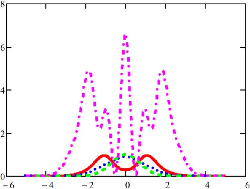
Evolution of the square modulus of an initial Gaussian function ruled by the heat-like Eq. (55); dash (t=0), dot (t=2), continuous (t=3), dash-dot (t=5).
The solution of Eq. (55) can be cast in the form:
Where the evolution operator in non-umbral form reads:
Thus considering, for example, a Hamiltonian of the type
The study of umbral evolutive PDE requires a more accurate analysis which cannot be comprised in the space of this concluding section. In this article we have gone through many aspects of symbolic calculus. Further results will be more thoroughly discussed elsewhere.
ACKNOWLEDGMENTS
The author expresses his sincere appreciation to Dr. Silvia Licciardi for the kind assistance during every stage of the article.
Footnotes
Namely
REFERENCES
Cite This Article
TY  - CONF
AU  - Giuseppe Dattoli
PY  - 2023
DA  - 2023/11/29
TI  - A Note on Low Factorial Based Polynomials
BT  - Proceedings of the 1st International Symposium on Square Bamboos and the Geometree (ISSBG 2022)
PB  - Athena Publishing
SP  - 85
EP  - 94
SN  - 2949-9429
UR  - https://doi.org/10.55060/s.atmps.231115.008
DO  - https://doi.org/10.55060/s.atmps.231115.008
ID  - Dattoli2023
ER  -


