
From Pythagoras to Fourier and From Geometry to Nature
DOI: https://doi.org/10.55060/b.p2fg2n.ch010.220215.013
Chapter 10. Waves and More
10.1 Relations to Chebyshev and Pseudo-Chebyshev Forms and to Fourier Series
The Gielis formula as generalization of Lamé curves and superellipses uses trigonometric functions which are transcendental. These equations can be rewritten in terms of Chebyshev polynomials [41, 46], for
There exists also a direct connection between pseudo-Chebyshev functions and flowers. Using Gielis transformations on Grandi or Rhodonea curves, but with
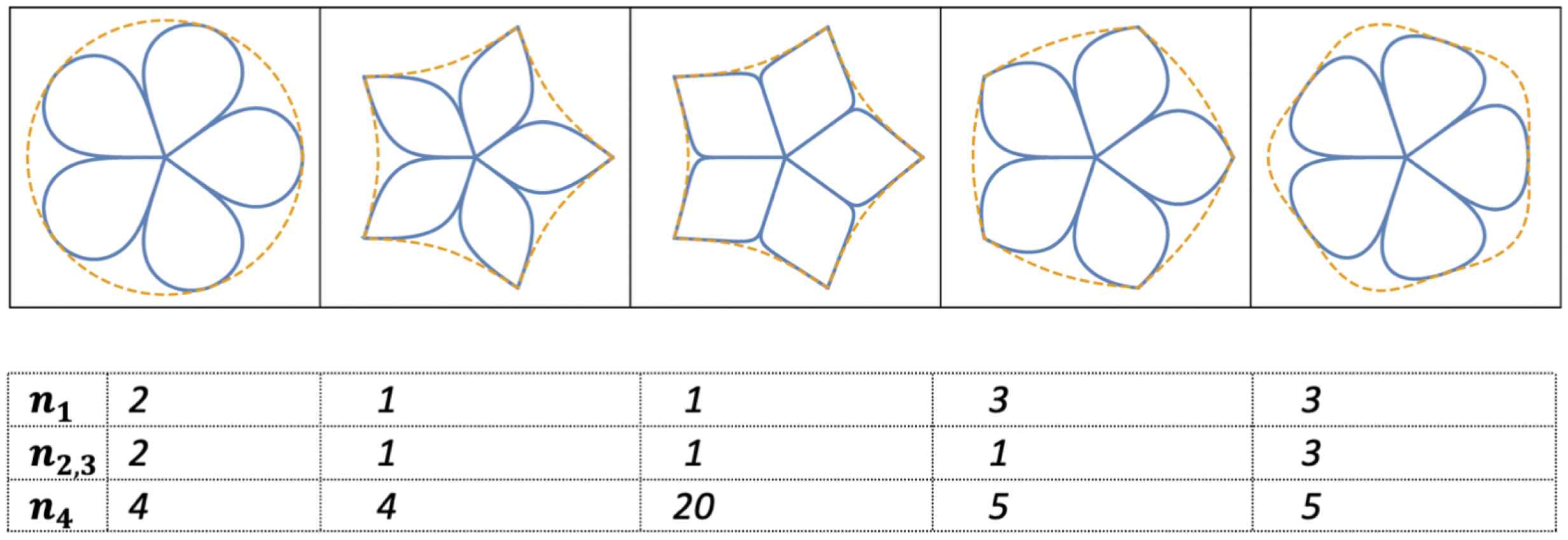
Equation (10.2) with
It is remarkable that flowers and leaves are connected to these polynomials and functions. Their multiple uses in mathematics can serve as a guide in the study of botany. For the study of flowers one can make use of the orthogonality properties of pseudo-Chebyshev functions [6].
This directly leads to Fourier series solutions using pseudo-Chebyshev functions of the fourth kind. Consider for an L1[−π, π], 2π-periodic function [6]:
Here Wn(x) is a pseudo-Chebyshev function of the fourth kind [6], which can be expressed using pseudo-Chebyshev functions of the first and second kind. A consequence of this result is that the partial sums of a Fourier series can be written in terms of pseudo-Chebyshev functions, as follows:
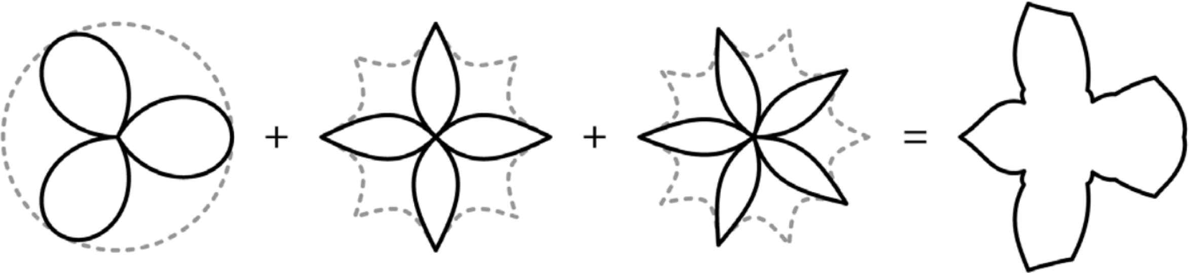
The flowers in Figure 27 can be understood as a single-term Grandi curve inscribed in a polygon defined by Equation (9.23). As a generalization of Fourier series (or trigonometric series in general) each individual term of a Fourier series can be transformed. One can define a generalized series, with ρ0, ρk defining a stretchable radius, as [45]:
Since the first constant term of the series ρ0a0 can be associated with a particular transformation ρ0, any shape described by Equation (9.23) is described precisely in one term of this generalized series ρ0a0 without any need for additional terms. Figure 28 shows a sum of three terms.
k-type Gielis curve with k = 3 for ρ(ϑ; f(ϑ), a, b, n1, n2, n3). The bird is the sum of ρ1(ϑ;
10.2 Coordinate Functions of First and Higher Order and Square Waves
Equation (9.23) and the generalized Fourier series of Equation (10.8) can be used to generate waves. One example is the generation of square waves. A square wave may be generated in various ways, e.g. with reference to step functions such as the Heaviside step function (Equation 10.9). Note that the Dirac delta function is the distributional derivative of the Heaviside function [43].
An alternative method is synthesis via Fourier series. One well-known disadvantage of this is the Fourier-Gibbs phenomenon, whereby oscillations occur in points of measure zero. These phenomena are an inherent feature of the method, but may be mediated in practice by using
In order to generate a square wave which is differentiable everywhere, all exponents in Equation (9.24) are equal to 1, m = 4 and A is very large, so that the cosine term becomes very small, ɛ. In Figure 29, the shape of the sine wave is given for various values of ɛ [43].
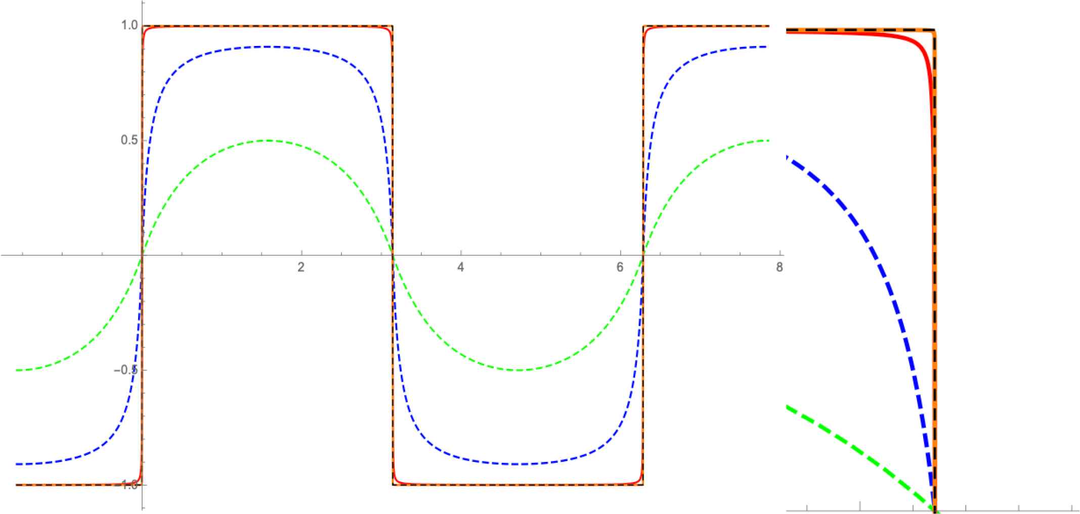
As long as ɛ is finite and not zero, the function is differentiable everywhere. In this way, Gibbs phenomena are avoided and differentiability can be ensured everywhere. These curves can also be framed in a window, e.g. the interval [−1; 1] or in a Gaussian window
Left: cosines for ɛ = 10−5 in Gaussian window with n = 2. Right: decaying square wave [43].
Second and higher order trigonometric functions based on Equation (9.23) can be generated. Given a shape ρ(ϑ) defined by Equation (9.23), the polar plot is generated by:
The functions c(ϑ) and s(ϑ) are displayed in Figure 31 with values A = 2, B = 1, m1 = 1.5, m2 = 0.5, n1 = 1, n2 = 2 and n3 = 3. This can be continued to any order.
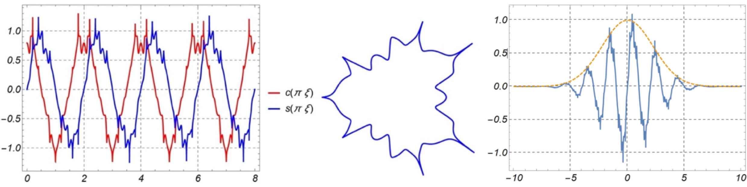
Supertrigonometric functions with associated polar graphs and the Gaussian version.
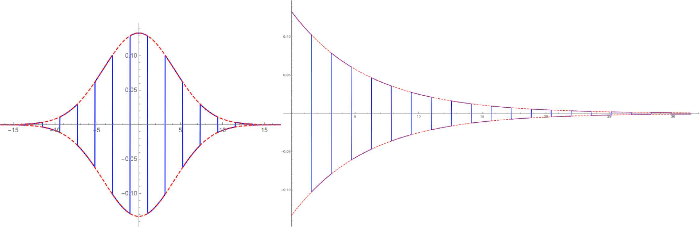
Figure 32 displays rational Gielis curves with m a rational number (m = 4/5). Increasing the values of the n2, n3 parameters lowers the magnitude of the main q-th harmonic partial (5th in this example) and raises the magnitudes of the other partials, as can be seen in the two harmonic spectra of the X-coordinates waveforms. The spectra of the Y-coordinates waveforms (not shown) have similar polyphonic spectral characteristics [27].
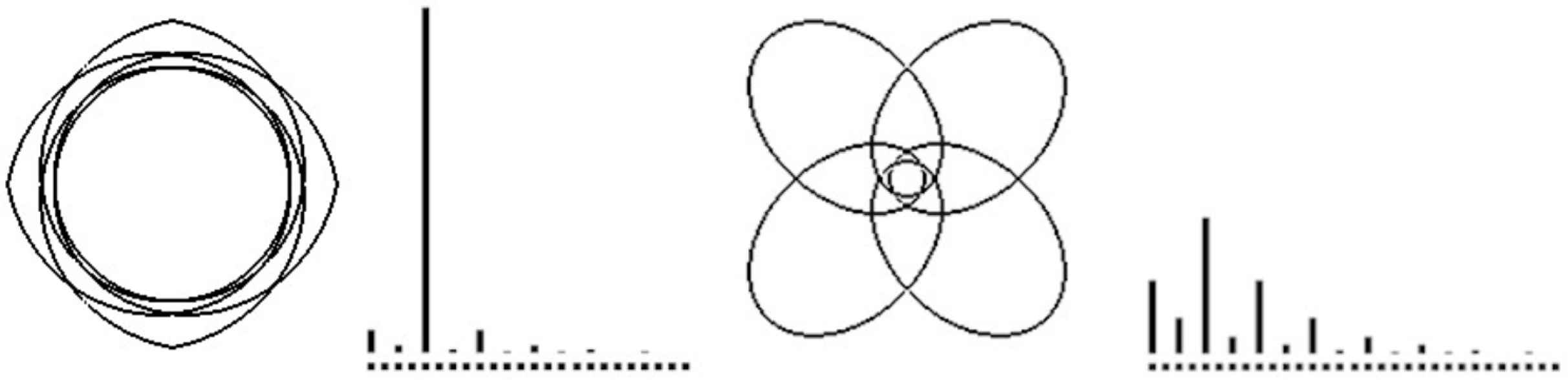
Polyphonic timbres inherent to Gielis curves with parameter values ρ(ϑ, 4/5, 1, 1, 1, 1, 1) (left) and ρ(ϑ, 4/5, 1, 1, 1, 9, 9) (right).
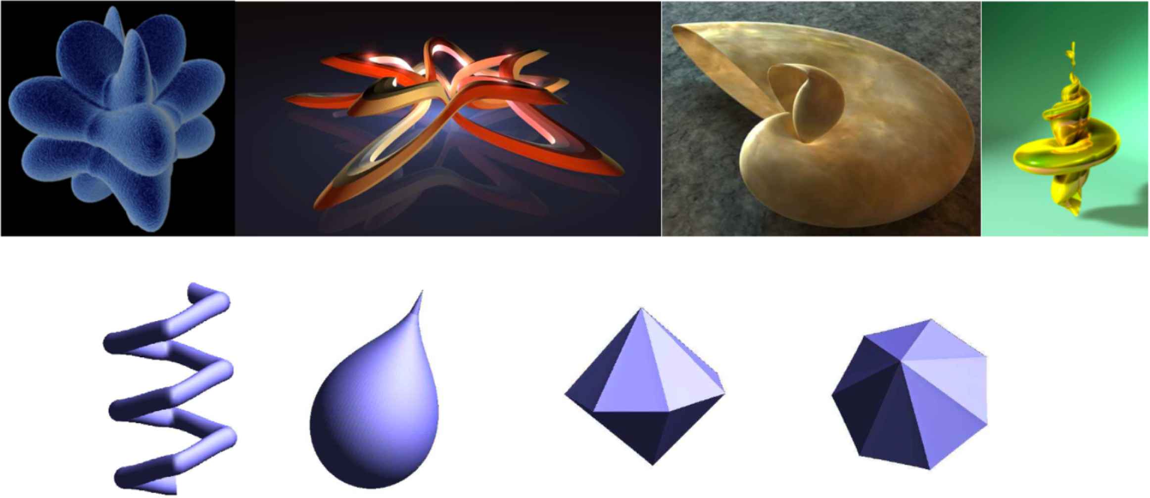
10.3 Higher Dimensions
Equation (9.23) can be extended to any dimension. In 3D, both spherical coordinates (Equation 10.13) [9] and parametric representations (Equation 10.14) can be used:
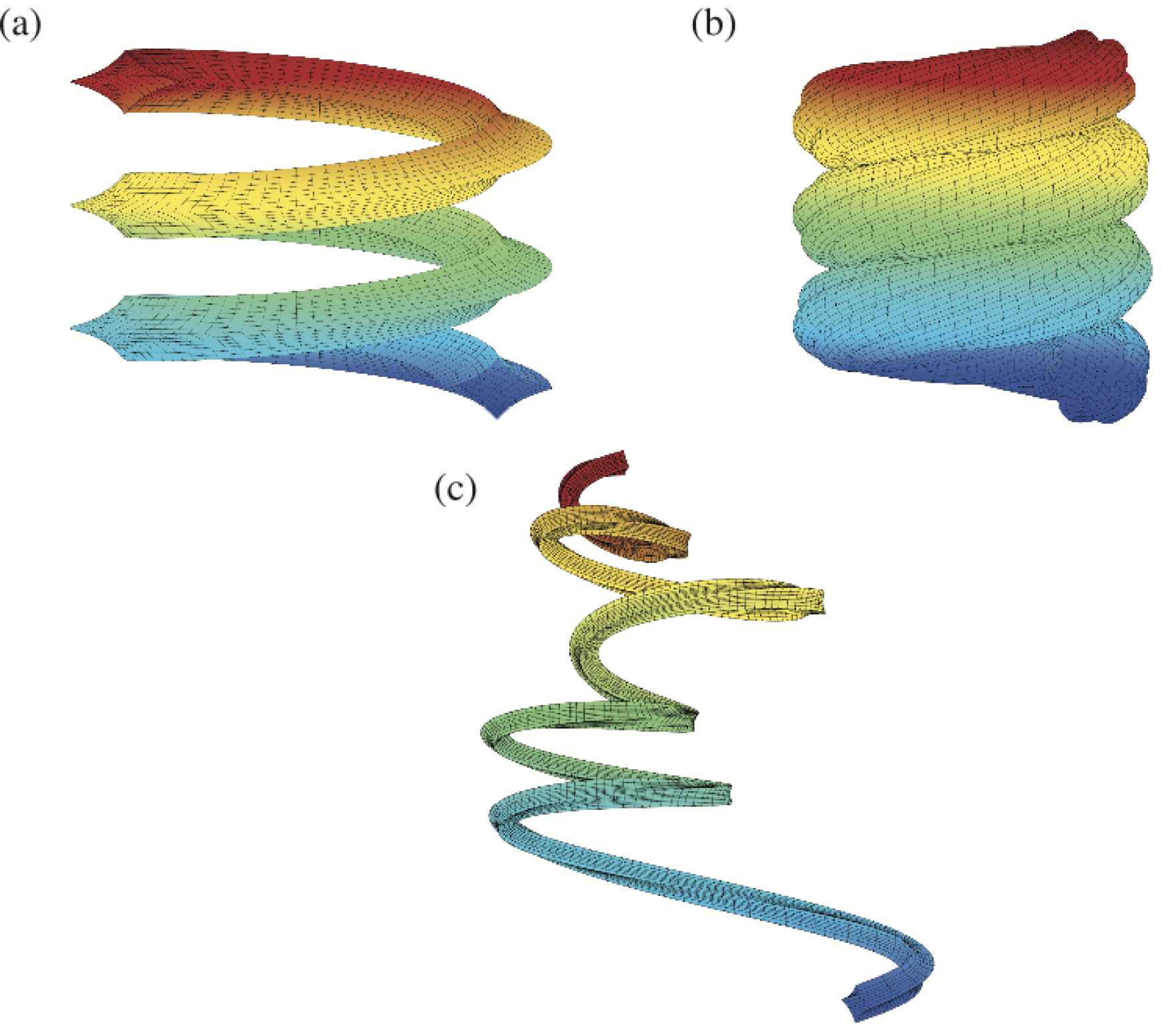
The parametric equation (10.14) is based on two perpendicular cross sections ρ1, ρ2 which can be of different sizes leading to toroidal structures (see Figures 33 & 34) [41]:
3D shapes defined by Equation (10.14).
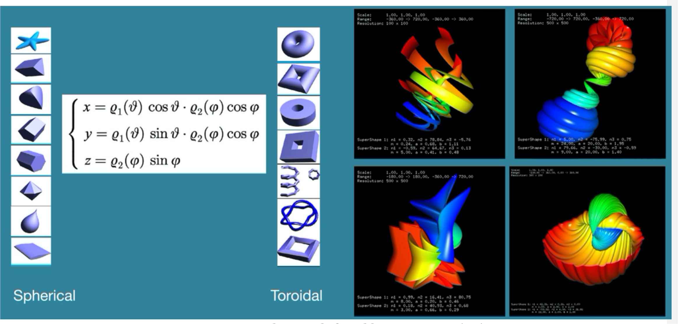
3D shapes defined by Equation (10.14).
This can be further extended within the framework of Generalized Möbius-Listing surfaces and bodies with Equations (10.15) and (10.16) [49, 96, 97]. Both the basic line and the cross section can be defined by any of the curves discussed earlier. The lower index of the notation
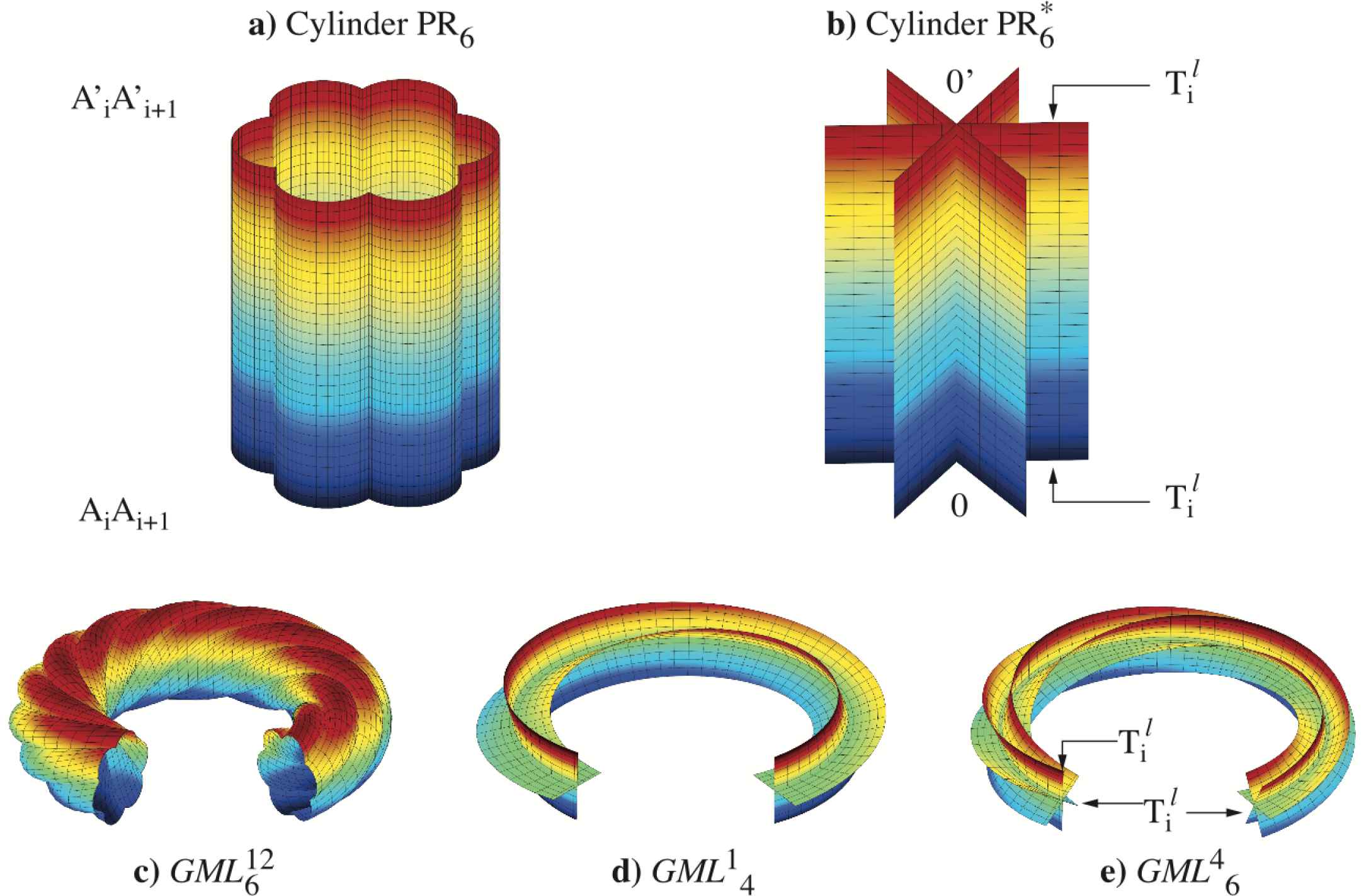
Prisms and
Generalized Rotating and Twisting bodies
The main advantage of such general coordinate systems, as also observed by Lamé, is that to each physical shape or phenomenon a best fitting coordinate system can be found. The goal of mathematical physics then is to solve the boundary value problems associated with the problem under investigation [41, 55].
Both the cross section and the basic line can be defined by Equation (9.24) and a time component can operate on cross section, basic line and twisting parameters for dynamical studies.
For more information, please contact us at:
info@athena-publishing.com


